Real Example of Data Processing and Exploratory Data Analysis with R

Introduction

This section illustrates an example of processing and analyzing data using R, focusing on the Zea mays (corn) experiment data from Charles Darwin’s studies. We will cover reading files from the file system, working with paths, manipulating data with tidyr and dplyr, generating summary statistics, and visualizing the results through plots to explore relationships between cross- and self-pollinated Zea mays plants.

About the Experiment

The data were presented in Charles Darwin’s book The Effects of Cross and Self Fertilization in the Vegetable Kingdom in 1876. He hypothesized that cross-pollination could make their offspring stronger (in terms of height, in his opinion back then). To show this idea, he planted 15 pairs of Zea mays, one by self-pollination and the other by cross-pollination. Each pair of observations was grown in the same pots, and there were a total of 4 pots in this study.

This study is famous not because of its contribution to plant biology and genetics; instead, it is a famous wrong experiment in statistics. Darwin’s incorrect calculation was later corrected by Ronald A. Fisher, a renowned biostatistician (and you will see his name throughout your university life, from genetics to hematology).

File System and Path of the File

Understanding the file system and specifying the correct path to your data files is crucial in R for successful data import. In this example, the zea_mays.csv file is located in a subdirectory named data within the current working directory of this project. The working directory is the default location where R looks for files if a full path is not specified.

To check your current working directory in R, you can use the following command:

As a side note, if you execute this line in a .Rmarkdown file, it will return the file path where the markdown file is located unless specified elsewhere.

In contrast, if you execute this line in the R terminal, it will return the default root path of your R system unless specified elsewhere.

File Path Tree Diagram

This diagram illustrates a simple file system structure to demonstrate absolute and relative paths.

/ (root)
├── home
│   └── user
│       ├── documents
│       │   ├── BIOF1001
│       │   │   ├── THIS_MARKDOWN.rmd
│       │   │   └── IMAGE.png
│       │   └── notes.txt
│       └── downloads
|           └── Zea_mays.csv
└── var

Absolute Path Examples

An absolute path starts from the root directory (/) and specifies the full path to a file or directory. A reminder: in a Windows system, you will find your file path using \ instead of / in your file explorer. In R, you need to transform these \s to / if you directly copy and paste the file path.

• Path to THIS_MARKDOWN.rmd: /home/user/documents/BIOF1001/THIS_MARKDOWN.rmd
• Path to Zea_mays.csv: /home/user/downloads/Zea_mays.csv

Relative Path Examples

A relative path is defined relative to the current working directory. It uses . to refer to the current directory, and .. means “go up one directory level”.

Assume that we are working on THIS_MARKDOWN.rmd, so the current directory is /home/user/documents/BIOF1001.

• Path to IMAGE.png from /home/user/documents/BIOF1001: ./IMAGE.png or IMAGE.png
• Path to Zea_mays.csv from /home/user/documents/BIOF1001: ../../Zea_mays.csv

Relative Path

In most projects you get from GitHub or other sources, you will typically see relative paths.

• What are the advantages and disadvantages of using absolute paths?
• What are the advantages and disadvantages of using relative paths?

Reading Zea mays Data

Now it’s your time to practice opening Zea_mays.csv using a relative path.

Solution

We can validate if you have correctly read the file by inspecting zea_mays:

Introducing tidyr and dplyr with Zea mays Example

In real-world examples, you might need to manipulate your dataframe to the right format for analysis or perform descriptive analysis of your data. Here, we introduce the tidyr and dplyr packages from the tidyverse collection, which provide powerful tools for these tasks.

Let’s install and load these packages if you haven’t already:

In the ecosystem of dplyr and tidyr, we use the concept of a pipeline: data is transformed step by step through functions. This transmission process is done using %>% operators, indicating that the dataframe will be the first argument of the next function.

flowchart LR
  A((Data)) -->|%>%| B[Function 1]
  B -->|%>%| C[Function 2]
  C --> E((Transformed data))

Pipeline Approach

The concept of a pipeline is widely used in programming languages. Even in Python, it is further integrated into machine learning algorithms.

• What are the benefits of using a pipeline?

Handling Messy Data

In real life, we might encounter human error and missing data in the dataset. Some common issues you might see:

• Missing data
• Wrong datatype
• Out of range

There are many techniques to handle these situations through statistical approaches, but here we use the simplest way: dropping them.

dplyr provides the function filter, which keeps the data that meets the filter condition:

• Removing rows with NA

• Removing out-of-range values

Identify Rows with Missing Values

Using the same techniques, you can do it in the opposite way to identify rows with potential errors. This is a critical skill when you are working with people who collect the data.

Using tidyr for Data Reshaping

The tidyr package helps in tidying data, making it easier to work with. For instance, if our Zea mays data were in a wide format (a table with many attributes in columns, i.e., self-pollinated heights and cross-fertilized heights, which are actually two observations), we could reshape it into a long format using pivot_longer. Although our current dataset might already be in a suitable format, here’s an illustrative example of how to use tidyr:

In this example, pivot_longer gathers the values from columns Cross.fertilized.plant and Self.fertilized.plant into a single column Height, with a new column Type indicating whether the height is from a cross- or self-pollinated plant.

An intuitive benefit of this transformation is that you can conduct regression analysis to analyze the association between fertilization type and height. You will learn how to do this in the future.

Using dplyr for Data Manipulation

The dplyr package offers functions for data manipulation such as filtering, selecting, mutating, and summarizing data. Let’s use dplyr to clean and prepare the Zea mays data for analysis. For instance, we can select specific columns or filter rows based on conditions:

Here, select chooses the columns Pair, Cross.fertilized.plant, and Self.fertilized.plant, and mutate creates a new column which is Cross.fertilized.plant minus Self.fertilized.plant.

Generating Summary Statistics of Zea mays Data

Once the data is prepared, we generate summary statistics to understand the distribution and characteristics of the variables. We can use base R functions or enhance our analysis with dplyr for grouped summaries.

This code provides a detailed summary by pollination type (Type), calculating the number of observations, mean height, standard deviation, and the range of heights for cross- and self-pollinated plants. The na.rm = TRUE argument ensures that missing values are ignored in calculations.

Plotting to Explore Relationships Between Cross- and Self-Pollinated Zea mays

Visualization is a key part of exploratory data analysis. We use the ggplot2 package to create various plots that compare the heights of cross-pollinated and self-pollinated Zea mays plants, exploring potential relationships and differences.

Boxplot for Comparison

A boxplot is useful for comparing the distribution of heights between the two pollination types.

This boxplot visually assesses the differences in growth between the two pollination methods, highlighting central tendencies, variability, and any potential outliers in the data.

Scatter Plot with Pair Information

Since the data includes paired observations (plants grown in pairs), a scatterplot with lines connecting pairs can illustrate individual differences within pairs.

This plot shows the height of each plant, with lines connecting the cross- and self-pollinated plants from the same pair, making it easier to see the direction and magnitude of differences within each pair.

Histogram for Distribution

Histograms can show the distribution of heights for each pollination type separately.

This histogram allows us to compare the distribution of height differences and see if there are notable patterns or central tendencies between cross- and self-pollinated plants.

Wrap-up

Through this analysis of the Zea mays dataset, we have demonstrated a comprehensive workflow in R for data analysis. Starting from understanding file systems and paths, reading data, manipulating data with tidyr and dplyr, generating detailed summary statistics, to creating various visualizations with ggplot2, this example underscores the importance of exploratory data analysis in understanding biological data.

Data Life Cycle Framework

At the end of this module, we introduce a higher-level overview of how to analyze data in the life sciences from a life cycle perspective. The idea of a data life cycle is widely used and applied in many fields. Griffin et al. (2018) proposed best practices in the life sciences. In this module, so far, we have covered a simple traditional approach to research data.

Data lifecycle, figure from Griffin et al. (2018)

Data Life Cycle and Examples

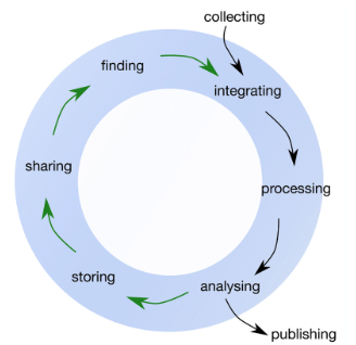
Life Cycle Stage	Example
Collecting	Read the data
Integrating	-
Processing	Manipulating tables
Analyzing	Reporting statistics
Publishing	Generating report and figures

References

Griffin, Philippa C, Jyoti Khadake, Kate S LeMay, Suzanna E Lewis, Sandra Orchard, Andrew Pask, Bernard Pope, et al. 2018. “Best Practice Data Life Cycle Approaches for the Life Sciences.” F1000Research 6: 1618.