Uniform Distribution
Yu Cheng Hsu
Intended learning outcomes
- Recognize and apply uniform distributions in statistical models
- Derive expected values of random variables
- Apply empirical probability mass functions in models
Describe a Distribution
Expectation
Definition
The expectation or mean of a random variable \(X\) with cdf \(F(X)\) and pdf \(f(x)\)
\[ \mathbb{E} (X) \triangleq \int xdF(x) = \begin{cases} \int_{-\infty}^{\infty} x f(x) dx \quad & \text{if }X\text{ is continuous} \\ \sum_{x \in \mathcal{X}} x f(x) \quad & \text{if }X\text{ is discrete} \end{cases} \]
provided that the integral or sum exists.
- If \(\mathbb{E}(X)= \infty\), we say that \(\mathbb{E} \left( X\right)\) does not exist.
Property of Expectation
Linearity
If \(X_1, . . . , X_n\) are random variables and \(a_1, . . . , a_n\) are constants, then
\[\begin{aligned}
\mathbb{E}[X_1+X_2] =\mathbb{E}[X_1] +\mathbb{E}[X_2] \\
\mathbb{E}[aX] =a\mathbb{E}[X]
\end{aligned}\]
Combining them to get the general form
\[ \mathbb{E}\big(\sum_i a_iX_i\big)=\sum_i a_i\mathbb{E}(X_i) \]
Analogy
Considering you are rolling two fair dice, the first time you get twice the points, and the second time you get the points shown
- What is the expectation of the first dice
- What is the expectation of the sum of first and second dice
Property of Expectation
Expected value of a constant
For any constant \(a \in \mathbb{R}\) ( i.e. in specific not a function of r.v ) the following holds \[ \mathbb{E} (a)= a \]
Proof
\[ \int a f(x)dx = a\int f(x)dx =a \]
Statistical independence
The following statement holds iff \(X\) and \(Y\) are statistically independent
\[ \mathbb{E}(XY)= \mathbb{E}(X)\mathbb{E}(Y) \]
Law of the unconscious statistician
Theorem: Let \(X\) be a random variable and let \(Y = g(X)\) be a function of this random variable.
\[\begin{cases} \mathrm{E}[g(X)] = \int_{\mathcal{X}} g(x) f_X(x) \, \mathrm{d}x \quad & \text{if }X\text{ is continuous} \\ \mathrm{E}[g(X)] = \sum_{x \in \mathcal{X}} g(x) f_X(x) \; . & \text{if }X\text{ is discrete} \end{cases}\]In a general term the following statement holds
\[ \mathrm{E}[g(X)] = \int_{\infty}^{\infty} g(x)\mathrm{d}F_X(x) \]
Variance
The variance measures the “spread” of a distribution
Definition
The variance of a random variable \(X\) is
\[ \sigma^2=\text{Var} \left( X \right) \triangleq \int (x-\mathbb{E}(x))^2dF(x)= \mathbb{E} \left[ \left( X - \mathbb{E}\left(X\right) \right)^2 \right] . \]
assuming this expectation exists
Discussion
Why does \(\mathbb{E}[X-\mathbb{E}(x)]\) not work as an indicator of “spreadness”?
This term is 0 \[ \begin{align} \mathbb{E}[X-\mathbb{E}(x)]=\mathbb{E}(X)-\mathbb{E}(x)=0 \end{align} \]
Property of Variance
\[ \begin{aligned} 1. \; &\mathbb{V}(X)=\mathbb{E}(X^2)-\mathbb{E}(X)^2 \\ 2. \; &\mathbb{V}(aX+b)=a^2\mathbb{V}(X) \\ 3. \; &\mathbb{V}\big(\sum_i a_iX_i\big)=\sum_i a_i^2\mathbb{V}(X_i) \end{aligned} \]
Proof:
\[ \begin{aligned} \mathbb{V}(X) = & \mathbb{E} \left[ \left( X - \mathbb{E}\left(X\right) \right)^2 \right] = \mathbb{E}[X^2-2X\mathbb{E}(X)+(\mathbb{E}(X)^2)]\\ = & \mathbb{E}(X^2)-2\mathbb{E}(X)^2+\mathbb{E}(X)^2 =\mathbb{E}(X^2)-\mathbb{E}(X)^2 \\ \mathbb{V}(aX+b) = & \mathbb{E}(a^2X^2+2abX+b^2)-(a^2\mathbb{E}(X)^2 +2ab\mathbb{E}(x)+b^2) \\ = & a^2\mathbb{E}(X^2)-a^2\mathbb{E}(X)^2 = a^2\mathbb{V}(X) \end{aligned} \]
Application:
Variance estimation for t-test with unequal variance
Property of Variance
Statistical independence
The following statement holds iff \(X\) and \(Y\) are statistically independent \[ \mathbb{V}(X+Y)=\mathbb{V}(X)+\mathbb{V}(Y) \]
Proof:
\[ \begin{aligned} \text{Assuming } & \mathbb{E}(X) \quad \&\quad \mathbb{E}(Y) = 0 \\ \mathbb{V}(X+Y)=&\mathbb{E}((X+Y)^2)=\mathbb{E}(X^2+2XY+ Y^2)\\ =&\mathbb{E}(X^2)+2\mathbb{E}(XY)+\mathbb{E}(Y^2)\\ =&\mathbb{E}(X^2)+2\mathbb{E}(X)(Y)+\mathbb{E}(Y^2)\\ =&\mathbb{E}(X^2)+\mathbb{E}(Y^2) \end{aligned} \]
Discrete vs. continuous random variables
For a random variable \(X\), we can categorize them into continuous random variables and discrete random variables
Discrete random variables
- Intuitive way:
- the sample space \(\Omega\) is a discrete space (countable)
- Official definition:
- cdf \(FX(x)\) is a step function of \(x\)
Continuous random variables
- Intuitive way:
- the sample space is a \(\Omega\) continuous space (uncountable)
- Official definition:
- cdf \(FX(x)\) is a continuous function of \(x\)
Wrap-up:
Uniform Distribution Family
Discrete Uniform Distribution
A random variable \(X\) with the sample space \(\Omega\) with \(N\) distinct elements \(\{x_a, \dots, x_b\}\). We write that X follows a discrete uniform distribution \(X \sim \text{Uniform}\left(N\right)\).
Properties
- Support: \(\{x_a\dots x_b\}\)
- Parameter: \(N\) number of distinct outcomes
- pmf
\[ \begin{aligned} P ( X = x) \; &= \; \frac{1}{N}, \quad x \in \Omega \end{aligned} \]
- Mean: \(\frac{a+b}{2}\)
Examples
- outcome of a fair coin flip
- outcome of a fair dice roll
- number on a drawn card from a well-shuffled deck
Continuous Uniform Distribution
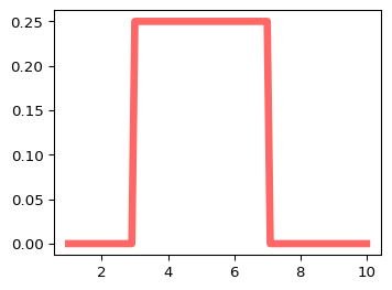
We write a random variable \(X\) follows a continuous uniform distribution over an interval \([a, b]\) as \(X \sim \text{Uniform}\left(a, b\right)\) if
Definition
Support: \([a,b]\)
Parameter: \(a,b\) range
pdf \[ f_X(x) = \begin{cases} \frac{1}{b - a} & \text{ if } x \in [a, b] \\ 0 & \text{otherwise} , \end{cases} \]
Mean: \((a+b)/2\)
Variance: \((b-a)^2/12\)
Example
Given \(X \sim \text{Uniform}(a, b)\), please show that
- \(\text{E} \left(X\right) = \frac{a+b}{2}\)
- \(\text{E} \left(X^2\right) = \frac{a^2 + ab + b^2}{3}\)
\[ \small \begin{align} \mathbb{E}(X) &= \int_{-\infty}^{\infty} x\, f_X(x)\, dx = \int_{a}^{b} x \cdot \frac{1}{b-a}\, dx = \frac{1}{b-a} \int_{a}^{b} x\, dx \\ &= \frac{1}{b-a} \left[ \frac{x^2}{2} \right]_{a}^{b} = \frac{1}{b-a} \left( \frac{b^2}{2} - \frac{a^2}{2} \right) = \frac{b^2 - a^2}{2(b-a)} = \frac{(b-a)(b+a)}{2(b-a)} \\[6pt] &= \frac{a+b}{2}. \end{align} \]
Example
Given \(X \sim \text{Uniform}(a, b)\), please show that for any number \(u,v,w\), which \(a<u<v<w<b\) and \(v-u=w-v=c\), please show that
\(\text{P} (u\leq X\leq v) = \text{P} (v\leq X\leq w)\)
\[ \begin{align*} \text{P} (u\leq X\leq v) &= P(x\leq v)-P(x\leq u) \\ &= \frac{v - a}{b - a}-\frac{u - a}{b - a}=\frac{c}{b-a}\\ \text{P} (v\leq X\leq w) &= P(x\leq w)-P(x\leq v) \\ &= \frac{w - a}{b - a}-\frac{v - a}{b - a}=\frac{c}{b-a} \end{align*} \]
Empirical distribution function
One application of axioms is their heuristic inspiration to create an empirical distribution from observed data. Given independent and identically distributed (iid) samples \(\{x_1, \ldots, x_N\}\) of random variable \(X\)
Definition
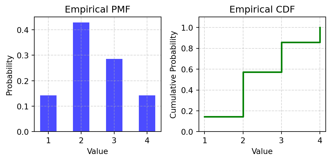
the empirical pmf for \(X\) is
\[ \hat{f}_N(x) = \frac{1}{N} \sum_{i=1}^N I(x_i = x) , \]
and the empirical cdf
\[ \hat{F}_N(t) = \frac{1}{N} \sum_{i=1}^N I(x_i \leq t) , \]
where \(I\) is the indicator function.
Example
Suppose we have observations \([1,2,2,2,3,3,4]\) Please plot the empirical pdf and cdf of the observations
Generating samples from empirical distribution
Assumption
The only random variables a computer can generate are \(X\sim\text{uniform}(0,1)\)
Problem
We want to generate random samples \(X\sim\text{uniform}(3,7)\)
Intuitive way
- Scaling the distribution to the width 4 \(X\rightarrow 4X\)
- Translate it from [0,4] to [3,7]: \(X \rightarrow 4X+3\)
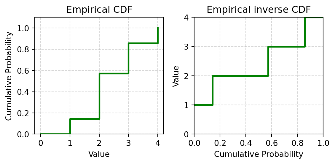
Inverse transform methods
What we are actually doing is calculating the inverse function of the CDF of \(X \sim \text{Uniform}(3,7)\).
- Recalling cdf of a uniform distribution is \(F(x)=\frac{x-a}{b-a} \quad \forall a\leq x \leq b\)
- The inverse cdf is \(F^{-1}(x)=(b-a)x+a\)
Plugging \(a=3,b=7\) we can get
\[F^{-1}(x)=4x+3\]
The thing we did is actually do the inverse function of CDF. This is the fundamental approach of generating random samples
Inverse transform methods
We can generate random number with its cdf \(F(x)\) through its inverse function \(F^{-1}(x) \quad \forall x \sim \text{uniform}(0,1)\)
\[ v = F^{-1}(x) \]
Example
Suppose we have observations \([1,2,2,2,3,3,4]\) Please plot the empirical cdf and inverse cdf of the observations
Checking Empirical distribution function fulfill axioms
Non-negativity
\[ \begin{aligned} \because N>0 \quad \& \quad I(x)\begin{cases} 1 \quad & \text{if }X\text{ is TRUE} \\ 0 \quad & \text{if }X\text{ is FALSE} \end{cases} \geq 0 \\ \rightarrow \hat{f}_N(x) = \frac{1}{N} \sum_{i=1}^N I(x_i = x) \geq 0 \end{aligned} \]
Unit measure
let the support has \(t\) unique values \(\{X_1 \dots X_t\}\) \[ P(X) = \sum_{t} \frac{1}{N} \sum_{i=1}^N I(x_i = X_t) = \frac{N}{N}= 1 \]
Intended learning outcomes
- Recognize and apply uniform distributions in statistical models
- Derive expected values of random variables
- Apply empirical probability mass functions in models
Why did the statistician join the army?
Because he heard they were looking for people who could fit into a strict Uniform !