Multivariate statistics
Yu Cheng Hsu
Intended learning outcomes
- Apply definitions and theorems regarding joint, conditional, and marginal distributions.
- Recognize and explain Simpson’s paradox.
Random vector
A more general term for defining random variables: suppose we have \(n\) random variables \(x_1, x_2, \dots, x_n\). We can arrange them into a (column) vector \(X\):
\[\begin{aligned} X=\begin{bmatrix} x_1\\ x_2\\ \vdots\\ x_n \end{bmatrix} = [x_1, x_2, ..., x_n ]^T \end{aligned} \]
Definition
An \(n\)-dimensional random vector is a mapping from a sample space \(\mathcal{S}\) to an \(n\)-dimensional Euclidean space \(\mathcal{R}^n\).
Joint probability function
Definition
Given a discrete bivariate random vector \(X=[x_1, x_2]\), the joint probability mass function (pmf) is defined by
\[ f_{X}(a, b) \; \triangleq \; P_{x_1, x_2} \left(x_1 = a, x_2 = b\right) . \]
As the name suggests, the joint pmf also satisfies the following axioms:
\[ f_{X, Y}(x, y) \ge 0 \quad \forall \, (x, y) \in \mathcal{R}^2 \]
And \[ \sum_{(x, y) \in \mathcal{R}^2} f_{X, Y}(x, y) = \sum_y\sum_x f_{X, Y}(x, y) = 1 . \]
Calculation of random vectors
Mean
\[ \small \begin{align} \mathbb{E}(X)=\begin{bmatrix} \mathbb{E}(X_1)\\ \mathbb{E}(X_2)\\ \vdots\\ \mathbb{E}(X_n) \end{bmatrix} = [\mu_1, \mu_2, ..., \mu_n ]^T =\mathbb{\mu} \end{align} \]
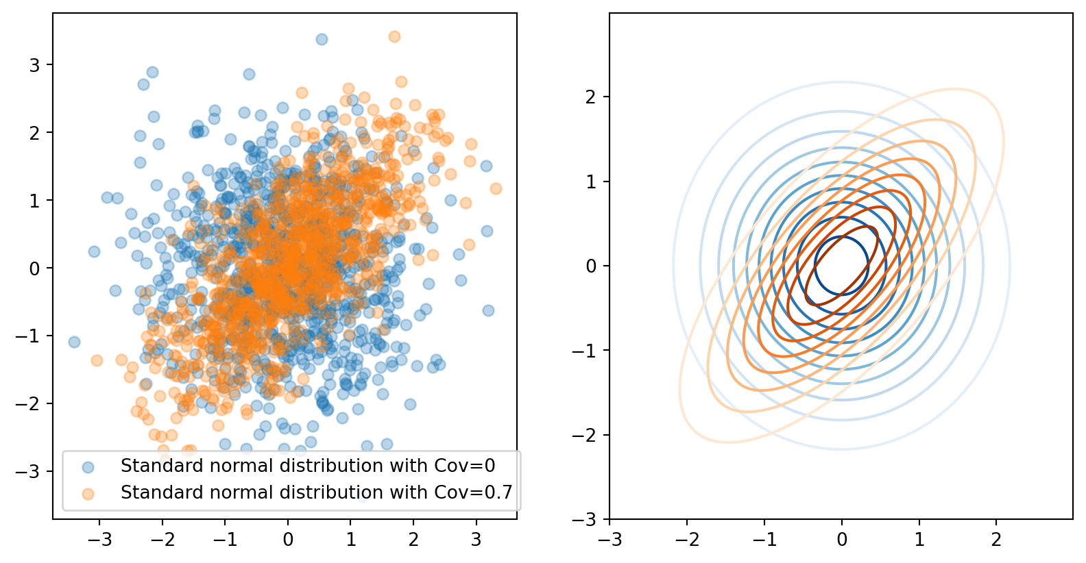
Variances and Covariances
\[ \small \begin{align} & \mathbb{E}((X-\mathbb{\mu})(X-\mathbb{\mu})^T) = \begin{bmatrix} \sigma_{11} & \sigma_{12} & \dots & \sigma_{1n} \\ \sigma_{21} & \sigma_{22} & \dots & \sigma_{2n} \\ \vdots & \vdots & & \vdots \\ \sigma_{n1} & \sigma_{n2} & \dots & \sigma_{nn} \end{bmatrix} = \mathbb{\Sigma} \\ & \text{ where } \sigma_{ii}=\mathbb{V}(X_i) \text{, and } \sigma_{ij}=cov(X_i,X_j) = \mathbb{E}((X_i-\mu_i)(X_j-\mu_j)) \end{align} \]
Example
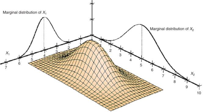
Marginal probability mass function
Definition
The marginal pmfs of random vector \(X=(x_1, x_2)\) are defined by
\[ \begin{cases} f_1(x_1) \; \triangleq \int_{\infty}^{\infty} \; f(x_1,x_2)d x_2, \quad f_2(x_2) \; \triangleq \int_{\infty}^{\infty} \; f(x_1,x_2)d x_1 \\ f_{x_1}(x_1) \triangleq \sum_{x_2 \in \mathcal{X_2}} f(x_1,x_2), \quad f_{x_2}(x_2) \triangleq \sum_{x_1 \in \mathcal{X_1}}f(x_1,x_2) \end{cases} \]
The reason why it is called marginal as it marginalize out the variables not of your concern
Example: Contingency table
Consider a randomized treatment-control study observing potential improvements in reducing cancer incidence rates:
| Cancer | Healthy | |
|---|---|---|
| Treatment | 3 | 97 |
| Control | 21 | 70 |
Questions:
- What is the marginal probability of developing cancer?
\(\frac{3+21}{3+97+70+21} = \frac{24}{191}\)
- What is the marginal probability of being selected for the treatment group?
\(\frac{3+97}{3+97+70+21} = \frac{100}{191}\)
Conditional probability
Definition
Given a random vector \((X, Y)\) if \(P(Y) > 0\), then
\[ P( X \mid Y ) \triangleq \frac{P(X \cap Y)}{P(Y)} . \]
Conditional probability distributions
With joint pdf \(f_{X,Y}(x,y)\) and marginal pdfs \(f_X(x)\) and \(f_Y(y)\), for any \(x\) such that \(f_X(x) > 0\), the conditional pdf of \(Y\) given that \(X = x\) is defined by
\[ f_{Y \mid X}( y \mid x ) = \frac{ f_{X,Y}(x,y) }{ f_X(x) } \]
Similarly, for any \(y\) such that \(f_Y(y) > 0\),
\[ f_{X \mid Y} \left( x \mid y \right) = \frac{ f_{X,Y}(x,y) }{ f_Y(y) } \]
Conditioning direction
Direction matters \[ P\left(Y \mid X=x \right) \]
The probability of \(y\) given that I have observed the random variable \(X=x\). Swapping the direction has a different implication:
Denominator is a scalar
\[ f_{Y \mid X}( y \mid x ) = \frac{ f_{X,Y}(x,y) }{ f_X(x) } \]
It is clear that the denominator is not a function of \(y\). From \(Y\)’s perspective, the denominator is a scalar. This is an important calculation step for the rest of the class.
Marginalization as an expectation of conditional probability
We can rewrite the equation for marginal probability as a product of conditional probability:
\[ f_X(X) = \int_{-\infty}^{\infty} \; f(x,y)dy = \int_{-\infty}^{\infty} \; f_{X \mid Y} ( x \mid y ) p_Y(y) dy = \mathbb{E}[f_{X \mid Y} ( x \mid Y )] \]
Example: Contingency table (again)
Consider a randomized treatment-control study observing potential improvements in reducing cancer incidence rates:
| Cancer | Healthy | |
|---|---|---|
| Treatment | 3 | 97 |
| Control | 21 | 70 |
Questions:
- What is the probability of developing cancer given that you are in the treatment group?
\(\frac{3}{100}=\frac{\frac{3}{191}}{\frac{100}{191}}\)
- What is the probability of developing cancer given that you are in the control group?
\(\frac{21}{91}=\frac{\frac{21}{191}}{\frac{91}{191}}\)
Statistical independence
Definition
Given a random vector \((X, Y)\), \(X\) and \(Y\) are independent if and only if (iff),
\[ f_{X, Y}(x, y) = f_X(x) f_Y(y) . \]
If \(X\) are \(Y\) are independent, we write \(X \perp Y\).
By this definition, it implies the following three properties:
\[ \small \begin{align} X \perp Y \; \Rightarrow \quad & f_{Y \mid X}(y \mid x) = f_Y(y) \\ & \mathbb{E}(XY) =\mathbb{E}(Y)\mathbb{E}(Y) \\ & \sigma_{xy}=0 \end{align} \]
Note: The converse of the last property is not always true.
Implication
- Independence = one event conveys no information about the other
- Independence does not mean mutually exclusive events.
Example: Contingency table (again..)
Consider a randomized case-control study observing potential improvements in reducing cancer incidence rates:
| Cancer | Healthy | |
|---|---|---|
| Treatment | 3 (a) | 97 (c) |
| Control | 21 (b) | 70 (d) |
Questions:
- If cancer development is independent from whether treatment was received, what could be the possible relationship of \(a, b, c, d\)?
\(\frac{a}{b}=\frac{c}{d}\) or \(\frac{a}{c}=\frac{b}{d}\)
- What is the implication for the effectiveness of the intervention if cancer development is independent from whether treatment was received?
Treatment does not reduce the chance of developing cancer
Simpson’s paradox
While the presence or absence of some confounding variable changes the probability distribution: \[ \frac{P\left( Y = 1 \mid X = x_1 \right) }{ P\left( Y = 1 \mid X = x_2 \right)} = c \]
However, conditioned on \(Z = z\) for some \(z\), \[ \frac{P\left( Y = 1 \mid X = x_1, Z = z \right) }{ P\left( Y = 1 \mid X = x_2, Z = z \right)} \neq \frac{P\left( Y = 1 \mid X = x_1 \right) }{ P\left( Y = 1 \mid X = x_2 \right)} \]
Example: Treatment of Kidney Stones?
A study by Bonovas and Piovani (2023) comparing open surgery versus percutaneous nephrolithotomy (PCNL) for treating kidney stones:
| Open Surgery | PCNL | |
|---|---|---|
| Success | 273 | 289 |
| fail | 77 | 61 |
Questions:
What is the probability of successfully removing a kidney stone if you undergo:
- Open Surgery \(\frac{273}{350}\)
- PCNL \(\frac{289}{350}\)
Based on the above probabilities, which surgery would you choose?
Percutaneous Nephrolithotomy (PCNL)
Example: Treatment of Kidney Stones?
In clinical practice, doctors usually perform PCNL for stone diameters less than 2 cm and open surgery for stone diameters greater than or equal to 2 cm.
| Open Surgery | PCNL | |
|---|---|---|
| Success | 81 | 234 |
| fail | 6 | 36 |
| Open Surgery | PCNL | |
|---|---|---|
| Success | 192 | 55 |
| fail | 71 | 25 |
Questions: Given that your stone diameter is less than 2 cm, what is the probability of successfully removing a kidney stone if you undergo:
Implication:
- Include all possible confounding variables in the analysis.
- Understand the context and how the data was collected.
Independence, association, and causal effects
Association (statistical dependence) is not causation.
From the overall table in the previous example, you might think that the type of surgery does not affect the outcome (Note that this is a causal claim).
But in reality the success or not also depends on the size of stone.
Implication
- Statistical dependencies are used to approximate causal effects by including possibly all confounders.
Bibliography Note
Bonovas, Stefanos, and Daniele Piovani. 2023. “Simpson’s Paradox in Clinical Research: A Cautionary Tale.” Journal of Clinical Medicine. MDPI.
Tacq, J. 2010. “Multivariate Normal Distribution.” In International Encyclopedia of Education (Third Edition), edited by Penelope Peterson, Eva Baker, and Barry McGaw, Third Edition, 332–38. Oxford: Elsevier. https://doi.org/https://doi.org/10.1016/B978-0-08-044894-7.01351-8.