Expectation-Maximization Algorithm
The Expectation-Maximization (EM) algorithm is an iterative method used to find the potential Maximum Likelihood Estimates (MLE) or Maximum a Posteriori (MAP) estimates of parameters in statistical models, specifically when the model depends on unobserved latent variables.
It is widely used in:
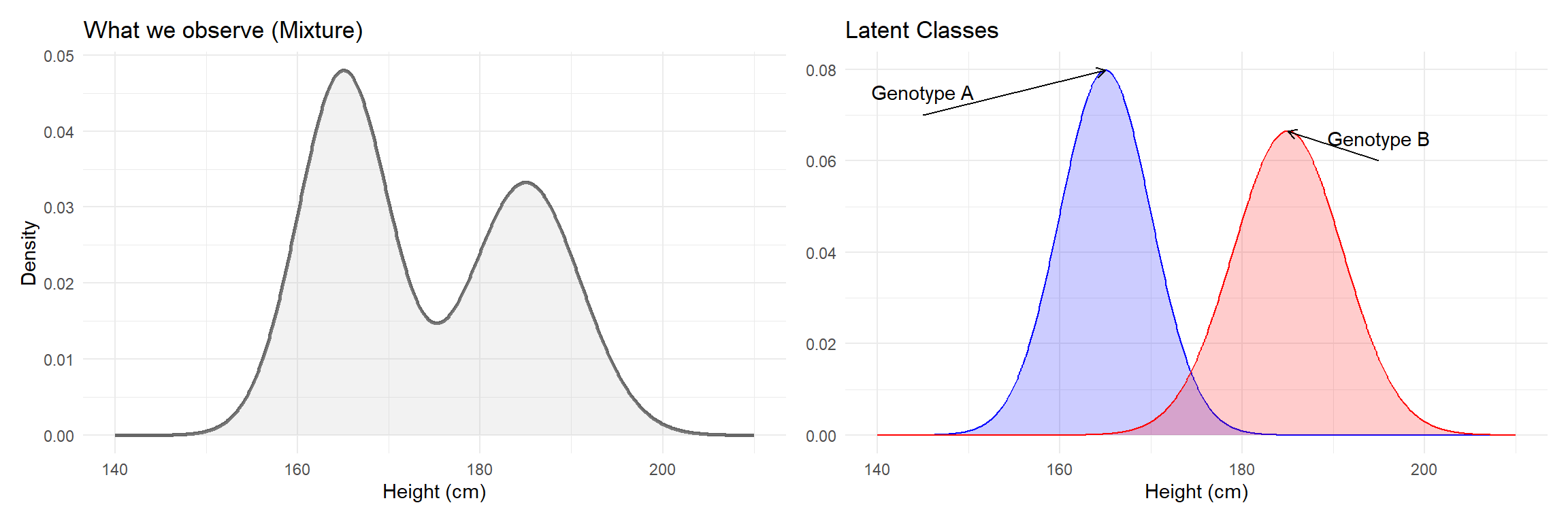
In real life, our observations might come from different subgroups (latent variables).
Example:
Height differences across different populations (e.g., Genotype/Ancestry).
Modeling an overall population mean and variance does not reveal the underlying differences among your observations.
General format
Suppose we have:
Our goal is to maximize the observed data likelihood: \[ \arg\max_\theta P(X | \theta) \]
Example
Goal: 1. Estimate the probability of each person belonging to a group. 2. Estimate the mean and variance for each group.
Directly maximizing the log-likelihood \(\ell(\theta; X)\) is difficult because:
\[ P(X | \theta) = \sum_Z P(X, Z | \theta) \] The summation (or integral) over \(Z\) occurs inside the logarithm of the likelihood function \(\log P(X|\theta)\).
Intuition:
Tricks: Pretend as if we know \(Z\) (latent) class
General format
Choose an initial guess for the parameters
Example
We initialize with
General format
Compute the responsibility of the latent variables given the data and current parameters: \[ \small \gamma =P(Z | X, \theta^{(t)}) \]
Then, use this to construct the Q-function (Responsibility X likelihood):
\[ \small \begin{aligned} & Q(\theta | \theta^{(t)}) \\ & = \sum_{Z} \log P(Z | X, \theta^{(t)}) P(X, Z | \theta) \end{aligned} \]
Example
For each person \(i\), we calculate the “responsibility” (posterior probability) of being Asian or European:
\[ \small \begin{aligned} & \gamma_{i,A} = P(\text{Asian} | x_i, \theta^{(t)}) \\ & \frac{p(x_i | \text{Asian}) p(\text{Asian})}{p(x_i | \text{Asian}) p(\text{Asian}) + p(x_i | \text{Euro}) p(\text{Euro})} \end{aligned} \]
Tricks
The likelihood of the observed data is a weighted average of different normal distributions. Calculate likelihood is unnecessary.
e_step <- function(X, mu_a, sigma_a, p_a, mu_e, sigma_e, p_e) {
  prob_x_given_a <- dnorm(X, mu_a, sigma_a)
  prob_x_given_e <- dnorm(X, mu_e, sigma_e)
  resp_a <- (prob_x_given_a * p_a) / (prob_x_given_a * p_a + prob_x_given_e * p_e)
  resp_e <- 1 - resp_a
  ll <- sum(log(p_a * prob_x_given_a + p_e * prob_x_given_e))
  return(list(resp_a = resp_a, resp_e = resp_e, ll = ll))
}
#| echo: true
def e_step(X, mu_a, sigma_a, p_a, mu_e, sigma_e, p_e):
prob_x_given_a = norm.pdf(X, mu_a, sigma_a)
prob_x_given_e = norm.pdf(X, mu_e, sigma_e)
resp_a = (prob_x_given_a * p_a) / (prob_x_given_a * p_a + prob_x_given_e * p_e)
resp_e = 1 - resp_a
ll = np.sum(np.log(p_a * prob_x_given_a + p_e * prob_x_given_e))
return resp_a, resp_e, llGeneral format
Find the new parameters \(\theta^{(t+1)}\) that maximize the Q-function: \[ \small \theta^{(t+1)} = \operatorname{argmax}_{\theta} Q(\theta | \theta^{(t)}) \]
Example
Using the responsibilities \(\gamma_{i,A}\) calculated in the E-step, we update the parameters. For example, the mean height for Asians:
\[ \small \begin{aligned} & \mu_A^{(t+1)} = \\ & = \frac{\sum_{i=1}^n \gamma_{i,A} x_i}{\sum_{i=1}^n \gamma_{i,A}} \end{aligned} \]
Similarly, we update:
m_step <- function(X, resp_a, resp_e) {
  sum_resp_a <- sum(resp_a)
  sum_resp_e <- sum(resp_e)

  mu_a <- sum(resp_a * X) / sum_resp_a
  mu_e <- sum(resp_e * X) / sum_resp_e

  sigma_a <- sqrt(sum(resp_a * (X - mu_a)^2) / sum_resp_a)
  sigma_e <- sqrt(sum(resp_e * (X - mu_e)^2) / sum_resp_e)

  p_a <- sum_resp_a / length(X)
  p_e <- 1 - p_a
  return(list(mu_a=mu_a, sigma_a=sigma_a, p_a=p_a, mu_e=mu_e, sigma_e=sigma_e, p_e=p_e))
}
#| echo: true
def m_step(X, resp_a, resp_e):
sum_resp_a = np.sum(resp_a)
sum_resp_e = np.sum(resp_e)
mu_a = np.sum(resp_a * X) / sum_resp_a
mu_e = np.sum(resp_e * X) / sum_resp_e
sigma_a = np.sqrt(np.sum(resp_a * (X - mu_a)**2) / sum_resp_a)
sigma_e = np.sqrt(np.sum(resp_e * (X - mu_e)**2) / sum_resp_e)
p_a = sum_resp_a / len(X)
p_e = 1 - p_a
return mu_a, sigma_a, p_a, mu_e, sigma_e, p_eGeneral format
Repeat steps 2 and 3 until the change in log-likelihood is below a threshold \(\epsilon\): \[|\ell(\theta^{(t+1)}) - \ell(\theta^{(t)})| < \epsilon\]
Typical choices for \(\epsilon\) are \(10^{-4}\) to \(10^{-6}\).
Example
Iterate until the parameters \(\mu, \sigma, p\) stabilize.
log_likelihoods <- c()
for (iteration in 1:10) {
  # E-Step
  results_e <- e_step(X, mu_a, sigma_a, p_a, mu_e, sigma_e, p_e)
  log_likelihoods <- c(log_likelihoods, results_e$ll)

  # M-Step
  results_m <- m_step(X, results_e$resp_a, results_e$resp_e)

  # Update parameters
  mu_a <- results_m$mu_a; sigma_a <- results_m$sigma_a; p_a <- results_m$p_a
  mu_e <- results_m$mu_e; sigma_e <- results_m$sigma_e; p_e <- results_m$p_e
}

cat(sprintf("Converged Means: Asian=%.2f, Euro=%.2f\n", mu_a, mu_e))
Converged Means: Asian=163.67, Euro=185.00Converged Mixing: p(Asian)=0.50Log-Likelihoods: -23.16991 -19.78781 -19.78747 -19.78747 -19.78747 -19.78747 -19.78747 -19.78747 -19.78747 -19.78747 #| echo: true
log_likelihoods = []
for iteration in range(10):
# E-Step
resp_a, resp_e, ll = e_step(X, mu_a, sigma_a, p_a, mu_e, sigma_e, p_e)
log_likelihoods.append(ll)
# M-Step
mu_a, sigma_a, p_a, mu_e, sigma_e, p_e = m_step(X, resp_a, resp_e)
print(f"Converged Means: Asian={mu_a:.2f}, Euro={mu_e:.2f}")
print(f"Converged Mixing: p(Asian)={p_a:.2f}")
print(f"Log-Likelihoods: {[round(x, 2) for x in log_likelihoods]}")