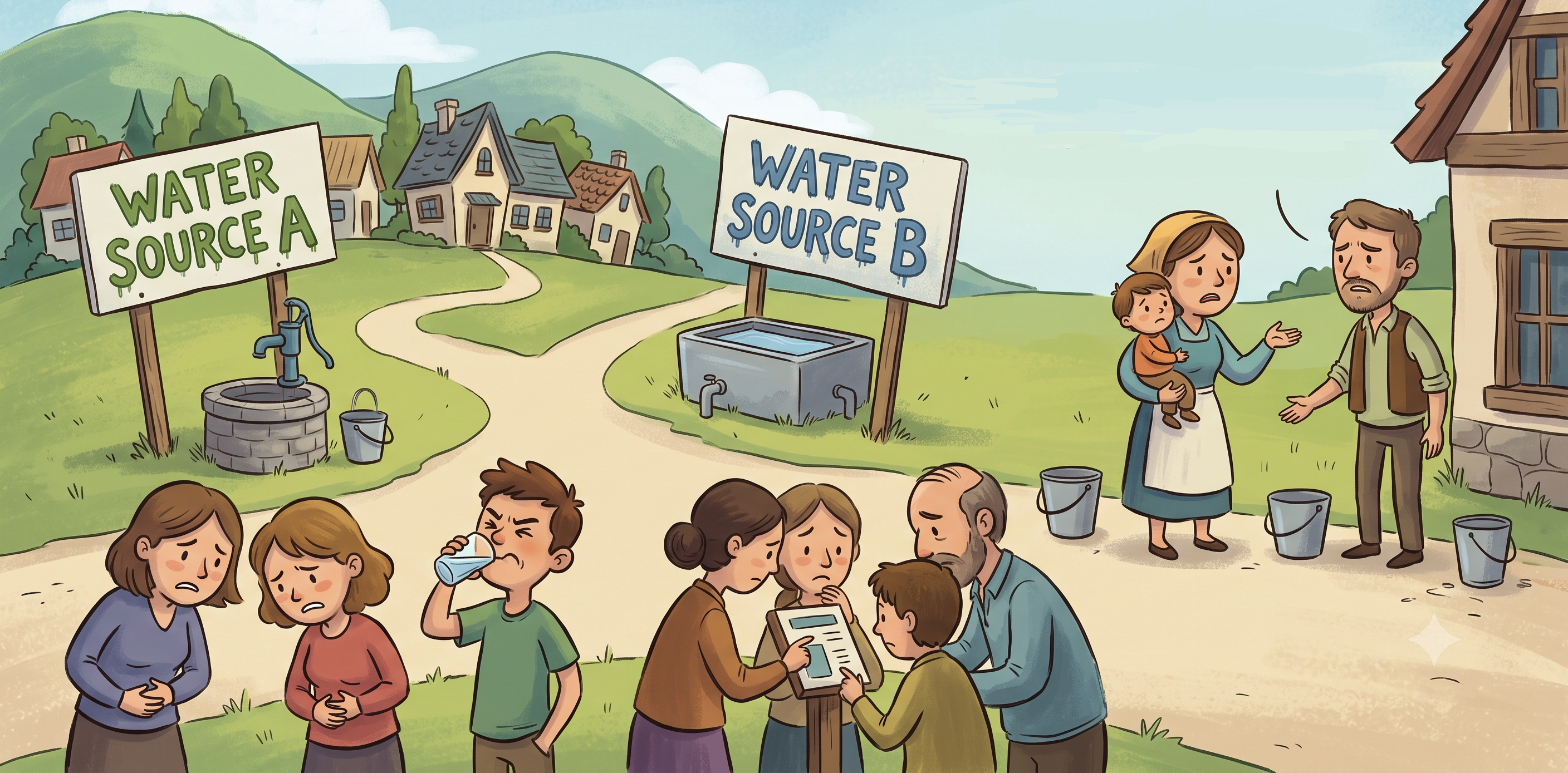
Epidemiology workshop

Yu Cheng Hsu

Learning objectives

• Analyze data from cohort study
• Analyze data from case-control study
• Justify the use cohort or case-control study

• Workshop background

In epidemiology, the “direction” of our data collection determines which statistical measures we can estimate. Today, we will use poker cards to simulate two study designs:

• Cohort study
• Case-control study

Set up

• Card back pattern = Exposure variable
  • Water Source A (Blue back)
  • Water Source B (Red back)
• Card face color = Outcome variable
  • Red card (hearts and diamonds): Infected
  • Black card (spades and clubs): Healthy

Cohort Study

Activity instruction

In a cohort study, we follow a specific population based on their exposure status to observe their future probability of developing a disease.

1. Everyone in the class: Showing only the card back (Water Source) and hiding the face.
2. Investigation: Leave your seat and find \(N\) residents from Area A and \(N\) residents from Area B.
3. Once you find your targets, ask them to reveal their card faces and record whether they are infected (Red card).
4. Record your data into the table below in r:

Cohort Study	Infected (Red)	Healthy (Black)
Water Source A (Exposed = \(N\))	a	b
Water Source B (Unexposed = \(N\))	c	d

Interpretation of cohort study

The fundamental question we can answer is:

Compared with the unexposed group, how likely is the exposed group to develop the disease (outcome)?

To answer this, we need to know

1. How likely is the outcome to occur in the unexposed group? (Risk)
2. How likely is the outcome to occur in the exposed group? (Risk)
3. Calculate the ratio of 2. to 1. (Relative Risk)

# Enter the data (a, b, c, d) you collected from your Cohort Study
a <- 5  # Number of infected in Area A (example)
b <- 3  # Number of healthy in Area A (example)
c <- 2  # Number of infected in Area B (example)
d <- 6  # Number of healthy in Area B (example)

# Calculate the Risk (Incidence)
risk_A <- a / (a + b)
risk_B <- c / (c + d)

# Calculate Relative Risk (RR)
RR <- risk_A / risk_B
cat("Relative Risk (RR) of the Cohort Study:", round(RR, 2), "\n")

Relative Risk (RR) of the Cohort Study: 2.5 

• RR represents “how many times more likely the exposed group is to develop the disease compared to the unexposed group.”

Inference on RR ¹

• \(\log(\text{RR})\) follows normal distribution with standard error (SE) \[ SE=\sqrt{\frac{1}{a}-\frac{1}{a+b}+\frac{1}{c}-\frac{1}{c+d}} \]

• Hypothesis \[ \begin{aligned} H_0: & \ln(RR) = 0 \\ H_a: & \ln(RR) \neq 0 \end{aligned} \]

• If your 95% Confidence Interval includes the number 0 (e.g., [-0.9, 2.4]), we fail to reject the Null Hypothesis, because \(\ln(RR) = 0\) is still a plausible reality.

1. This part is not included in the exam for the following reason: 1. Z-test is an approximation method that does not reveal the true probability, 2. There is a more efficient and generalizable approach for adjusting for other variables.

Interpretation

• RR = 1 and log(RR) = 0: No difference in risk between groups
• RR > 1 and log(RR) > 0: Increased risk in the exposed group
• RR < 1 and log(RR) < 0: Decreased risk in the exposed group

# 1. Calculate the natural log of RR
log_RR <- log(RR)

# 2. Calculate the Standard Error (SE) for log(RR)
# The mathematical formula for the variance of log(RR) is:
# (1/a) - (1/(a+b)) + (1/c) - (1/(c+d))
se_log_RR <- sqrt((1/a) - (1/(a+b)) + (1/c) - (1/(c+d)))

# 3. Build the 95% Confidence Interval on the log scale
# (using Z = 1.96)
ci_lower_log <- log_RR - 1.96 * se_log_RR
ci_upper_log <- log_RR + 1.96 * se_log_RR

# 4. Exponentiate [ exp() ] back to the normal RR scale
ci_lower <- exp(ci_lower_log)
ci_upper <- exp(ci_upper_log)

# Print the results
cat("Relative Risk (RR):", round(RR, 2), "\n")

Relative Risk (RR): 2.5 

cat("95% CI: [", round(ci_lower, 2), ",", round(ci_upper, 2), "]\n")

95% CI: [ 0.67 , 9.31 ]

Case-Control Study

Activity instruction

In a case-control study, we start with people who already have the disease and compare them with people who do not have the disease based on their past exposure.

1. Everyone in the class: Show only the card face (hearts, clubs, etc.) and hide the card back.
2. Investigation: Leave your seat and find \(N\) infected individuals (Cases, Red cards) and \(N\) healthy individuals (Controls, Black cards).
3. Once you find your targets, ask them to reveal their card back and record which water source they lived near.
4. Record your data in R:

Case-Control Study	Cases (Infected = N)	Controls (Healthy = N)
Lived near Water Source A	a	b
Lived near Water Source B	c	d

Interpretation of Case-Control study

We are trying to answer a similar question as the cohort study, but the sampling is different.

Key difference from cohort studies

• We cannot estimate risk directly from a case-control study because the ratio of cases to controls is set by the study design.
• Relative risk (RR) is not directly estimable from this design.

1. Odds of disease among exposed individuals: \(a/b\)
2. Odds of disease among unexposed individuals: \(c/d\)

We use the odds ratio (OR) \[ \frac{a/b}{c/d} = \frac{a \times d}{b \times c} \] to quantify the association between exposure and outcome.

# Enter the data you collected from your Case-Control Study
disease_data_cc <- matrix(
  c(6, 3,   # Area A: Cases (a), Controls (b) (example)
    2, 5),  # Area B: Cases (c), Controls (d) (example)
  nrow = 2,
  byrow = TRUE
)

# Calculate the odds of disease
Odds_A <- disease_data_cc[1,1] / disease_data_cc[1,2]
Odds_B <- disease_data_cc[2,1] / disease_data_cc[2,2]

# Calculate Odds Ratio (OR)
OR <- Odds_A / Odds_B
cat("Odds Ratio (OR) of the Case-Control Study:", round(OR, 2), "\n")

Odds Ratio (OR) of the Case-Control Study: 5 

• OR represents “the strength of association between an exposure (e.g., a risk factor or treatment) and an outcome (e.g., a disease)”

Inference on OR

• Hypothesis

\[ \begin{aligned} H_0: & \text{OR} = \frac{\frac{a}{b}}{\frac{c}{d}} = 1 \\ H_a: & \text{OR} = \frac{\frac{a}{b}}{\frac{c}{d}} \neq 1 \end{aligned} \]

This is equivalent to evaluate \[ \frac{a}{b} = \frac{c}{d} \]

• We can use Fisher’s Exact Test to test it

# Use Fisher's Exact Test to calculate the OR and P-value
result_cc <- fisher.test(disease_data_cc)
cat("Odds Ratio (OR) of the Case-Control Study:", round(result_cc$estimate, 2), "\n")

Odds Ratio (OR) of the Case-Control Study: 4.47 

cat("P-value:", signif(result_cc$p.value, 3), "\n")

P-value: 0.315 

Interpretation

• OR = 1 and log(OR) = 0: Exposure is not associated with the outcome
• OR > 1 and log(OR) > 0: Exposure is positively associated with the outcome
• OR < 1 and log(OR) < 0: Exposure is negatively associated with the outcome

Discussion: how should I determine the experiment design

While case-control and cohort studies have similarities, they are rarely interchangeable due to practical reasons:

• Sample size considerations
• Ability to handle rare events
• Practical implementation
• Level of evidence

The “Needle in a Haystack” Problem: Rare Diseases

Imagine you are investigating a very rare type of cancer that affects only 1 in 100,000 people.

Cohort Study design:

• Sample size: Large population (e.g., 500,000 people)
• Tracking time: Long period (if prospective cohort)
• Disease case rate: low

Case-Control design:

• Sample size: Relatively small (\(N\) disease vs. \(N\) healthy)
• Time: Not a major consideration
• Disease case rate: Not applicable

Takeaway:

• Case-control studies are economically feasible for studying rare diseases.
• The OR approximates the RR when the disease is rare.

(Optional) OR approximate to RR

Let’s recall the formulas using our \(2 \times 2\) table counts (\(a\) = Exposed Cases, \(b\) = Exposed Controls, \(c\) = Unexposed Cases, \(d\) = Unexposed Controls).

Relative Risk (RR): \[ \small RR = \frac{\text{Risk in Exposed}}{\text{Risk in Unexposed}} = \frac{\frac{a}{a+b}}{\frac{c}{c+d}} \]

Odds Ratio (OR):

\[ \small OR = \frac{\text{Odds in Exposed}}{\text{Odds in Unexposed}} = \frac{\frac{a}{b}}{\frac{c}{d}} = \frac{a \times d}{b \times c} \]

If a disease is extremely rare (e.g., 1 in 10,000 people), the number of sick (\(a\) and \(c\)) is incredibly tiny compared to the healthy people (\(b\) and \(d\)).

If \(a\) is vanishingly small, then adding it to \(b\) barely changes anything. Therefore the following approximation holds \[ \small \begin{aligned} a \ll b \implies & a + b \approx b \\ c \ll d \implies & c + d \approx d \end{aligned} \]

2. The “Unique Group” Problem: Rare Exposures

In contrast, we are studying the health effects of a chemical spill inside a specific, small battery factory.

Cohort Study design:

• Sample size: Manageable (\(N\) exposure v.s. \(N\) non-exposure)
• Tracking Time: depends

Case-Control design:

• Sample size: Large population required to identify enough exposed individuals

Takeaway:

• Cohort studies are usually a better choice for studying Rare Exposures.

Implementation Realities: Time, and Memory

Beyond statistical theory, study design is heavily dictated by human behavior and logistics.

• Recall Bias (Case-Control):
  • Rely on people’s memories to know the exposure.
  • e.g. If you ask a mother whose baby was born with a defect (Case) if she ate anything unusual during pregnancy
• Loss to follow-up (Cohort):
  • There is a risk of losing track of people.
  • e.g. If you track people for 10 years, participants may move away, change contact details, or drop out of the study.
  • If those who drop out differ systematically from those who stay, the results can be biased.

Implementation Realities: Finding good control

• Identifying a proper control group can be challenging

Pancreatic cancer and coffee MacMahon et al. (1981)

• Pancreatic cancer patient (case) v.s. Gastric ulcer (Hospital control)
• Hidden issue: Gastric ulcer patients are often advised to limit intake of irritants such as caffeine.
• Conclusion: Coffee intake appeared positively associated with pancreatic cancer.

GLP-1 and other medications Schuemie et al. (2019)

• Studies try to show the effect of GLP-1 therapies (once used for type 2 diabetes, now repurposed for weight control and cardiovascular risk reduction)
• Because of the variety of products, patients may not know whether they are taking the medication or not

Wrap up Summary

Feature	Cohort Study	Case-Control Study
Starting Point	Exposure (e.g., Water Source)	Disease (e.g., Gastroenteritis)
Direction of Time	Forward (Prospective)*	Backward (Retrospective)
Best Used For…	Rare Exposures	Rare Diseases
Primary Metric	Relative Risk (RR)	Odds Ratio (OR)
Biggest Risk	Loss to follow-up, Expensive	Recall bias, Hard to pick good controls

Learning objectives

• Analyze data from cohort study
• Analyze data from case-control study
• Justify the use cohort or case-control study

Optional materials - Connection with regression

Helper function

To perform regression analysis we need to transform our contingency table to proper dataframe

Helper function

# Helper fundtion to transform contingency table to dataframe
table_to_df <- function(contingency_table) {
  
  # Getting cell from the contingency table
  a <- contingency_table[1, 1] 
  b <- contingency_table[1, 2] 
  c <- contingency_table[2, 1] 
  d <- contingency_table[2, 2] 
  
  # Matching a, b, c, d to disease status and exposure
  Disease_Status <- c(rep(1, a), rep(0, b), rep(1, c), rep(0, d))
  Exposure_Status <- c(rep(1, a), rep(1, b), rep(0, c), rep(0, d))
  
  # Combine as dataframe
  df <- data.frame(
    Exposure = Exposure_Status,
    Disease = Disease_Status
  )
  
  return(df)
}

Cohort and Poisson regression

Consider the Exposure of A (X, 0 = control, live in B, 1 = exposure live in A), in Poisson regression, it is written as

\[ \ln(\text{Risk}) = \beta_0 + \beta_1 X \]

• \(\beta_0\): is the baseline log-risk (Intercept, baseline for the not exposed group).
• \(\beta_1\): the increase \(\ln(\text{Risk})\) due to exposure

Why \(\small\beta_1\) is the \(\small\log\text{(RR)}\)

1. Risk for living near Water Source A, and B \[ \small \log(\text{Risk}_A )= \ln\left(p_A\right) = \beta_0 + \beta_1, \quad \log(\text{Risk}_B )= \ln\left(p_B\right) = \beta_0 \]

2. Subtracking each 2, we will get

\[ \begin{aligned} \text{RR} = & \ln\left(\frac{\text{Risk}_{X=1}}{\text{Risk}_{X=0}}\right) = \ln(\text{Risk}_{X=1}) - \ln(\text{Risk}_{X=0}) \\ & = (\beta_0 + \beta_1) - \beta_0 = \beta_1 \end{aligned} \]

Perform the task in Poisson regression manner

Transforming to dataframe

# 2. transform contingency table DataFrame
disease_data_ch<- matrix(
  c(a, b,   # Area A: Cases (a), Controls (b) (example)
    c, d),  # Area B: Cases (c), Controls (d) (example)
  nrow = 2,
  byrow = TRUE
)
patient_data <- table_to_df(disease_data_ch)

# 3. inspect first 5 rows
head(patient_data, 5)

  Exposure Disease
1        1       1
2        1       1
3        1       1
4        1       1
5        1       1

Performing Poisson regression

# 4. perform Poisson regression
poisson_model <- glm(Disease ~ Exposure, 
                    data = patient_data, 
                    family = poisson(link = "log"))
summary(poisson_model)

Call:
glm(formula = Disease ~ Exposure, family = poisson(link = "log"), 
    data = patient_data)

Coefficients:
            Estimate Std. Error z value Pr(>|z|)  
(Intercept)  -1.3863     0.7071  -1.961   0.0499 *
Exposure      0.9163     0.8366   1.095   0.2734  
---
Signif. codes:  0 '***' 0.001 '**' 0.01 '*' 0.05 '.' 0.1 ' ' 1

(Dispersion parameter for poisson family taken to be 1)

    Null deviance: 11.574  on 15  degrees of freedom
Residual deviance: 10.245  on 14  degrees of freedom
AIC: 28.245

Number of Fisher Scoring iterations: 5

Case-control and logistic regression

Consider the Exposure of A (X, 0 = control, live in B, 1 = exposure live in A), in logistic regression, it is written as:

\[ \ln\left(\frac{p}{1-p}\right) = \beta_0 + \beta_1 X \]

• \(\beta_0\): baseline log-odds intercept (affected by the sampling ratio in case-control studies).
• \(\beta_1\): the log(OR) for living in A.

Implication

We can use logistic regression to analyze case-control study.

Why \(\small\beta_1\) is the \(\small\log\text{(OR)}\)

1. First we normalize the 2 by 2 table by its row sum

Case-Control Study	Cases (Infected = N)	Controls (Healthy = N)
Lived near Water Source A	a/(a+b) = \(p_A\)	b/(a+b) = \(1-p_A\)
Lived near Water Source B	c/(c+d) = \(p_B\)	d/(c+d) = \(1-p_B\)

2. Odds for living near Water Source A, and B \[ \small \log(\text{Odds}_A )= \ln\left(\frac{p_A}{1-p_A}\right) = \beta_0 + \beta_1, \quad \log(\text{Odds}_B )= \ln\left(\frac{p_B}{1-p_B}\right) = \beta_0 \]

3. Subtracking each 2 in 2. we will get

\[ \small \log(OR)= \ln\left(\frac{\frac{p_A}{1-p_A}}{\frac{p_B}{1-p_B}}\right) = \beta_1 \]

Perform the task in logistic regression manner

Transforming to dataframe

# 2. transform contingency table DataFrame
patient_data <- table_to_df(disease_data_cc)

# 3. inspect first 5 rows
head(patient_data, 5)

  Exposure Disease
1        1       1
2        1       1
3        1       1
4        1       1
5        1       1

Performing logistic regression

# 4. perform logistic regression
glm_model <- glm(Disease ~ Exposure, data = patient_data, 
                 family = binomial)
summary(glm_model)

Call:
glm(formula = Disease ~ Exposure, family = binomial, data = patient_data)

Coefficients:
            Estimate Std. Error z value Pr(>|z|)
(Intercept)  -0.9163     0.8367  -1.095    0.273
Exposure      1.6094     1.0954   1.469    0.142

(Dispersion parameter for binomial family taken to be 1)

    Null deviance: 22.181  on 15  degrees of freedom
Residual deviance: 19.833  on 14  degrees of freedom
AIC: 23.833

Number of Fisher Scoring iterations: 4

Historical notes

• In some old paper researchers tend to use logistic regression for cohort study.
  • Benefits
    • Intuitive
  • Pitfalls
    • Over-estimation on CI (Poisson are modeling frequency not binary outcomes)

This issue is solved by Zou (2004), and since them Poisson regression and logistic regression will get the exact same results in this context.

Bibilography notes

MacMahon, Brian, Stella Yen, Dimitrios Trichopoulos, Kenneth Warren, and George Nardi. 1981. “Coffee and Cancer of the Pancreas.” New England Journal of Medicine 304 (11): 630–33.

Schuemie, Martijn J, Patrick B Ryan, Kenneth KC Man, Ian CK Wong, Marc A Suchard, and George Hripcsak. 2019. “A Plea to Stop Using the Case-Control Design in Retrospective Database Studies.” Statistics in Medicine 38 (22): 4199–4208.

Zou, Guangyong. 2004. “A Modified Poisson Regression Approach to Prospective Studies with Binary Data.” American Journal of Epidemiology 159 (7): 702–6.