Introduction to R

Intergrative mini project

Yu Cheng Hsu

Learning goal

  • Designing analysis pipeline from experiment
  • Applying R to perform data analysis

Background: Darwin’s Experiment

  • Source: The Effects of Cross and Self Fertilization in the Vegetable Kingdom by Charles Darwin in 1876.
  • Hypothesis: Cross-pollination could make their offspring stronger (in terms of height).
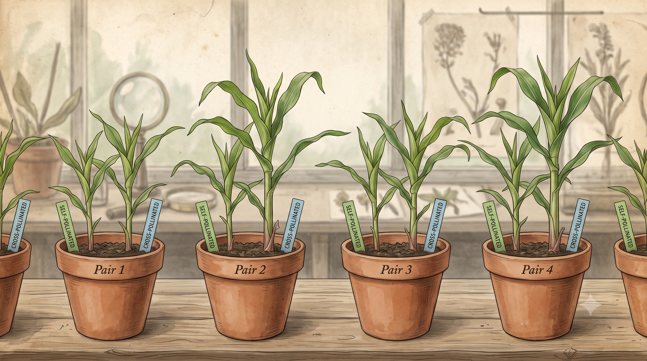
  • Experiment deisgn
    • 15 pairs of corn,
      • one by self-pollination
      • one by cross-pollination.
    • Each pair of observations was grown in the same pots,
    • 4 pots in this study.

Illustration of experiment design

Illustration of experiment design

The Data Science Workflow

Before diving into the code, let’s look at the roadmap. Every robust data science project follows a structured life cycle.

As a professional scientist to

  • Translate the experiment into actionable analysis plan
    • Outline the potential plan on
      • Processing
      • Analysis
      • Visualization
  • Convey the scientific findings

Project Roadmap

Some potential steps we need to perform:

  1. Data Import & Inspection: Load the experiment data and ensure data integrity.
  2. Data Manipulation (Processing): Calculate the height difference, capturing the paired experimental design.
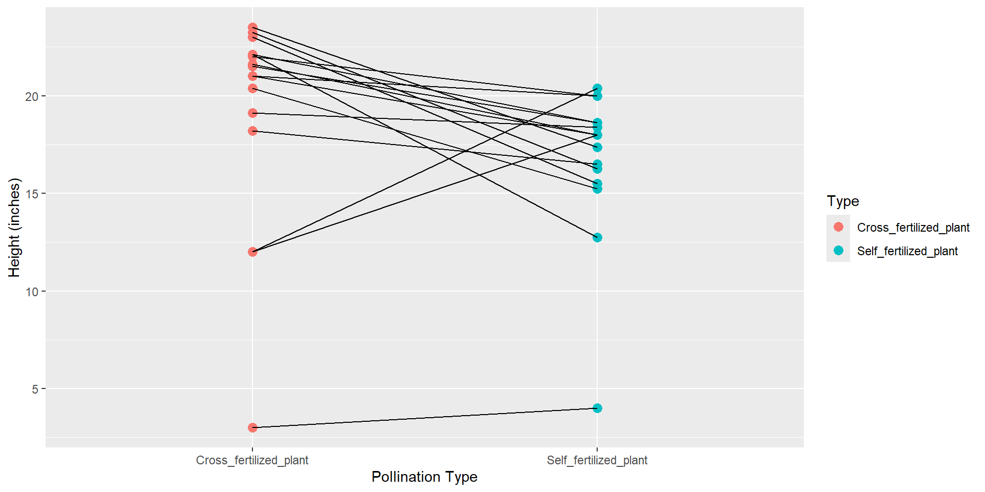
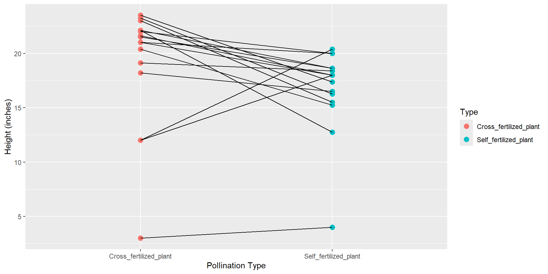
  3. Exploratory Data Analysis (EDA): Visualize the paired nature of the plants and the distribution of their height differences.
  4. Statistical test: Formulate our hypothesis and conduct statistical inference
  5. Conclusion & Reporting: Interpret the statistical output (p-value, mean difference).

Data Import and Inspection

Before any analysis, the absolute first step is to inspect the data to ensure its integrity.

Something you need check before you do anything:

  • Missing values
  • Typos and human errors
  • Data structures
# Load necessary libraries and the dataset
library(tidyverse)
zea_mays = read.csv("../../../assets/data/real-example/zea_mays.csv", header = TRUE)
head(zea_mays)
  Pots Pair Cross.fertilized.plant Self.fertilized.plant
1 Pot1    1                 23.500                17.375
2 Pot1    2                 12.000                20.375
3 Pot1    3                 21.000                20.000
4 Pot2    4                 22.000                20.000
5 Pot2    5                 19.125                18.375
6 Pot2    6                 21.500                18.625

Inspecting Data

# Check the data structure and look for missing values
## Apparently you can use zea_mays %>% anyNA() and so on
str(zea_mays)
'data.frame':   17 obs. of  4 variables:
 $ Pots                  : chr  "Pot1" "Pot1" "Pot1" "Pot2" ...
 $ Pair                  : int  1 2 3 4 5 6 7 8 9 10 ...
 $ Cross.fertilized.plant: num  23.5 12 21 22 19.1 ...
 $ Self.fertilized.plant : num  17.4 20.4 20 20 18.4 ...
anyNA(zea_mays) # Returns FALSE if there are no missing values
[1] TRUE
  • There is NA data being identified
zea_mays %>% 
  filter(is.na(Cross.fertilized.plant) | is.na(Self.fertilized.plant))
  Pots Pair Cross.fertilized.plant Self.fertilized.plant
1 Pot6   NA                     NA                    NA

Data wrangling plan

After inspecting the data here are some data wrangling (manipulation) works need to be done

  1. Handeling missing data
  2. Make a long tabke so that Each observation (Zea mays) must have its own row.
    1. Currently there are two observations in a row

And you will see the reasons later on

Removing Missing Data

Let’s remove the broken pairs before calculating our differences.

Good practice of coding

# 1. Drop any incomplete pairs
zea_mays <- zea_mays %>% 
  drop_na()
# 2. Verify the clean-up was successful
anyNA(zea_mays)
[1] FALSE

Not recommended way

# Not recommended approach
zea_mays <- zea_mays[-1,]
# 2. Verify the clean-up was successful
anyNA(zea_mays)
  • Try to avoid hard code on specific columns, rows by indexing

Reasons

  • Not robust to the change of data
  • Hard to understand the intention of the code

Data Preparation for Analysis

For our visual and statistical analysis, we need to calculate the true biological signal we care about: the height difference within each pair. We will also pivot the data for plotting.

# Calculate the paired difference
zea_mays <- zea_mays %>%
  mutate(diff.height = Cross.fertilized.plant - Self.fertilized.plant)

# Reshape for visualization
zea_mays_long <- zea_mays %>%
  pivot_longer(cols = c(Cross.fertilized.plant, Self.fertilized.plant), 
               names_to = "Type", values_to = "Height")

Analysis and Visualization

Scatter Plot with Pair Information

ggplot(zea_mays_long, aes(x = Type, y = Height, group = Pair)) +
  geom_point(aes(color = Type), size = 3) +
  geom_line(color = "grey") +
  labs(title = "Paired Heights of Zea mays", x = "Pollination Type", y = "Height (inches)") +
  theme_minimal()

The Wrong Approach: Paired t-test

We have 30 plants in total. Let’s see what happens if we adopts Darwin’s way’ (i.e. wrong statistical test).

  • The Wrong Approach: Independent t-test

Hypothesis: \[ \begin{aligned} H_0: & \mu_{\text{cross}} \leq \mu_{\text{self}} \\ H_a: & \mu_{\text{cross}} > \mu_{\text{self}} \end{aligned} \]

# INCORRECT: Running an unpaired 
# (independent) t-test
t.test(zea_mays$Cross.fertilized.plant, 
       zea_mays$Self.fertilized.plant, 
       alternative = "greater",
       paired = FALSE)

    Welch Two Sample t-test

data:  zea_mays$Cross.fertilized.plant and zea_mays$Self.fertilized.plant
t = 1.406, df = 27.048, p-value = 0.08555
alternative hypothesis: true difference in means is greater than 0
95 percent confidence interval:
 -0.5046025        Inf
sample estimates:
mean of x mean of y 
 19.11406  16.72656 

The Right Approach: Paired t-test

The problem with Darwin’s fallacy is that

  • Zea mays in the same pot shared
    • Same nutritient
    • Same weather condition

Violating the independent sample assumption of t-test. The corrected way is proposed by Ronald Fisher

Hypothesis: \[ \begin{aligned} H_0: & \mu_{\text{diff}} \leq 0 \\ H_a: & \mu_{\text{diff}} > 0 \end{aligned} \]

# CORRECT: Running a paired t-test
t.test(zea_mays$Cross.fertilized.plant, 
       zea_mays$Self.fertilized.plant, 
       alternative = "greater",
       paired = TRUE)

    Paired t-test

data:  zea_mays$Cross.fertilized.plant and zea_mays$Self.fertilized.plant
t = 2.0549, df = 15, p-value = 0.02887
alternative hypothesis: true mean difference is greater than 0
95 percent confidence interval:
 0.3507378       Inf
sample estimates:
mean difference 
         2.3875 

Discussion on the results

  • Using wrong statistical test could draw opposite interpretation
    • Darwin: \(p=0.086\) (Fail to reject \(H_0\))
    • Fisher: \(p=0.029\) (Reject \(H_0\))
  • Cross fertilization could make the plant bigger
  • Limitation of the experiments
    • Control of genotypes
    • Sample size

A full picture of analytics

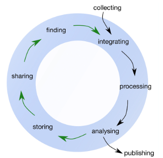
Griffin et al. (2018) proposed best practices in the life sciences. In this module, so far, we have covered a simple traditional approach to research data.

Data lifecycle, figure from Griffin et al. (2018)

Data lifecycle, figure from Griffin et al. (2018)
Life Cycle Stage Example
Collecting Read the data
Integrating -
Processing Manipulating tables
Analyzing Reporting statistics
Publishing Generating report and figures

Readinig list

Acknowledge

This case is inspired and adopted from Ross (2017)

Bibilography notes

Griffin, Philippa C, Jyoti Khadake, Kate S LeMay, Suzanna E Lewis, Sandra Orchard, Andrew Pask, Bernard Pope, et al. 2018. “Best Practice Data Life Cycle Approaches for the Life Sciences.” F1000Research 6: 1618.
Ross, Sheldon M. 2017. Introductory Statistics. Academic Press.