Cancer cell population monitoring

An ecology perspective

Yu Cheng Hsu

Intended learning outcomes

• Bullet point one
• Bullet point two
• Bullet point three

Project background

Tumor evolution

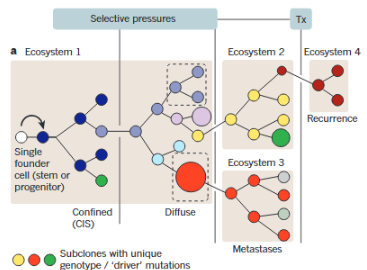
Tumor grows and evolves under evolution pressure

• Trophic
• Metabolic
• Immunological
• Therapeutic

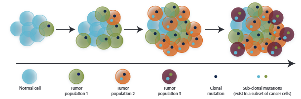
Intratumor heterogeneity (ITH), diversity in genetics, phenotypic or even epigenetic profiles, could equip tumor cells to adapt to different selection pressures.

Consequences of ITH

• Therapeutic failure
• Drug resistance

Intratumor heterogeneity of tumor cells from Walsh (n.d.)

Implication of ITH - Treatment

• ITH implies that tumor cells could (Darwinian):
  • Possess a genetic reservoir (accumulating different variations).
  • Adapt to different evolutionary pressures.
• Treatment is a selective evolutionary pressure (therapeutic pressure).
• Natural selection favors treatment-resistant tumor cells.

Selective pressure and drug resistance, image from Greaves and Maley (2012)

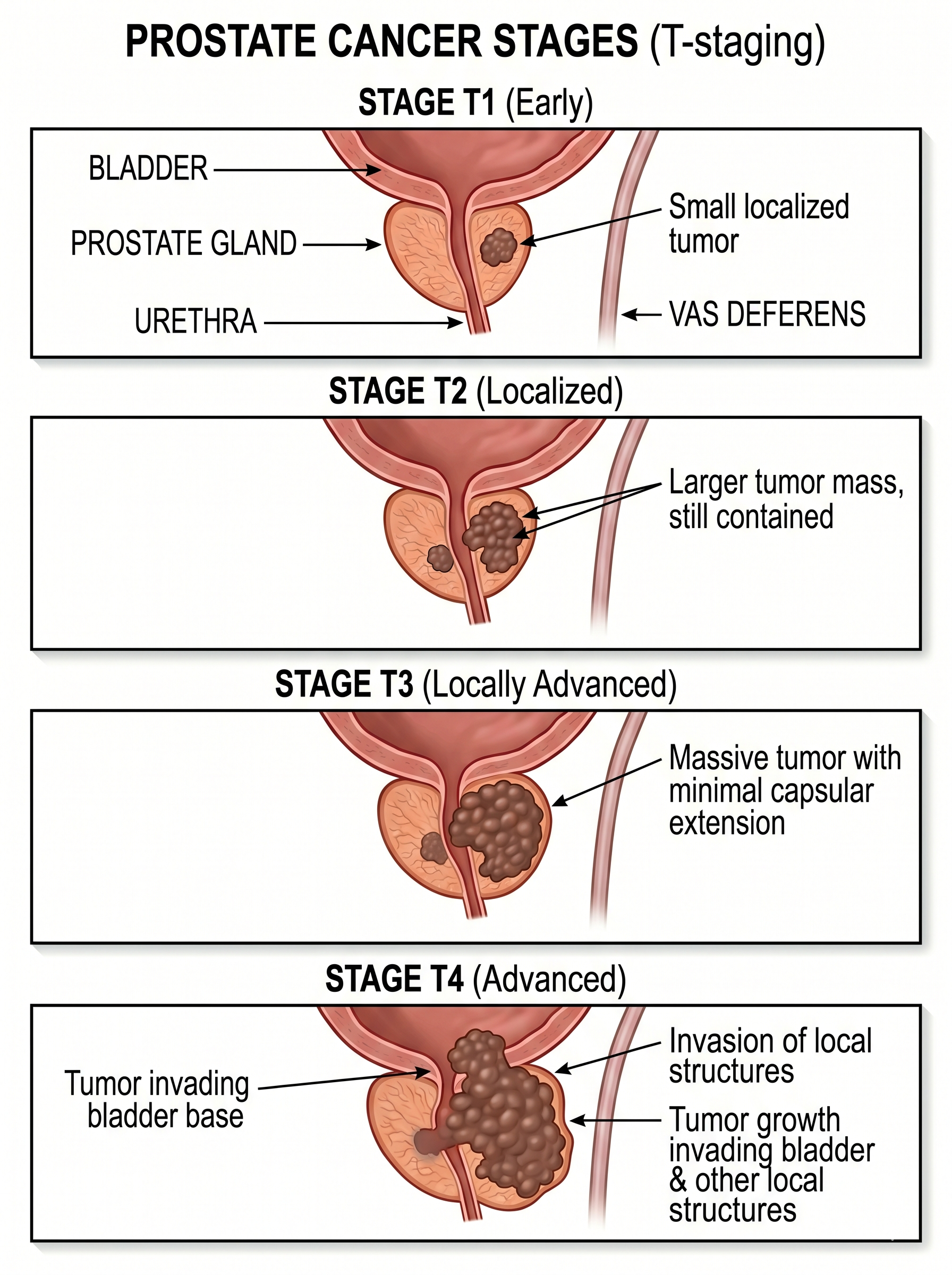
Prostate Cancer

Prostate Cancer in Hong Kong In 2023

• Prevalence rate (crude): 88.2 per 100K
• Mortality rate (crude): 15 per 100K

Treatment

• Radiotherapy
• Surgery
• Chemotherapy
• Hormone therapy
  • Prostate cancers are usually androgen-dependent. Hormone therapy works by reducing/blocking androgens, which can slow down or stop the growth of the cancer.

Prostate cancer

Hormone therapy for prostate cancer

• Androgen deprivation therapy (ADT) is used for advanced prostate cancer
• Continuous ADT
  • Disadvantages
    • Side effects (e.g., hot flashes, loss of libido)
    • Drug resistance (e.g., castration-resistant prostate cancer)
• Intermittent ADT (IADT)
  • Advantages Perera et al. (2020)
    • Delayed drug resistance
    • Reduced side effects (Improved quality of life)

Data sources

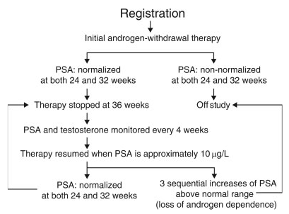
Bruchovsky et al. (2006) implemented a clinical trial of IADT

• Total participants: 103 eligible patients with prostate cancer
• Monitoring biomarkers:
  • Prostate-specific antigen (PSA) levels (indicates the activity of prostate cancer cells)
  • Testosterone (Effectiveness of ADT)
• Treatment protocol:
  • ADT is given for a fixed time (36 weeks) until PSA levels drop to 4 \(\mu\)g/mL
  • ADT is stopped until PSA levels rise to 10 \(\mu\)g/mL

IADT protocol, image from Bruchovsky et al. (2006)

Modeling ecology dynamics

Preface

• Predicting the population in the
  • microbiome
  • cells (tumors, donor-recipient interactions)

The idea of using these models is to estimate the potential growth of the cells of interest and provide insights into the underlying mechanisms of growth.

The modeling techniques in this topic are largely borrowed from ecology, where the study of species populations is of crucial interest:

• Interactions between species
• Environment

Simple model of tumor growth

A simple model to describe the change in a tumor cell population (\(\frac{dC}{dt}\)) is

\[ \frac{dC}{dt}=gC(t)-dC(t)=\alpha C(t) \]

• \(g\) is the growth rate of the tumor cells
• \(d\) is the death rate of the tumor cells
• \(\alpha\) is the net growth rate of the tumor cells

Implication of the simple model

• The population of the tumor cells at time \(t\) can be expressed as \[ C(t) = C(0)e^{\alpha t} \]

• If \(\alpha > 0\), the population will grow exponentially.
• If \(\alpha < 0\), the population will decline exponentially.
• If \(\alpha = 0\), the population will remain constant.

Limitations

• The model assumes that growth and death rates are constant over time, which may not be true in reality.
• The model does not account for interactions with other cell types or the environment.
• The model assumes there is no maximum population in a given environment.

Redesigning the model

From empirical observation, the growth of tumor cells usually follows these steps:

1. Starting rapid growth from a single/small collections of cells
2. The growth slows down as the population increases
3. Eventually, the population reaches a plateau

How to redesign the model

1. The growth rate is not constant; it is negatively proportional to the population size.
2. At a large enough population size, the growth rate will be zero.

Logistic growth model

An improved version of the simple model is the logistic growth model, which can be expressed as:

\[ \frac{dC}{dt}= \alpha(1-\frac{C(t)}{K}) C(t) \]

• \(K\) is the carrying capacity of the environment, which is the maximum population size that the environment can sustain.
• \(\alpha\) is the intrinsic growth rate of the tumor cells.

Qualitative inspection of the logistic growth model

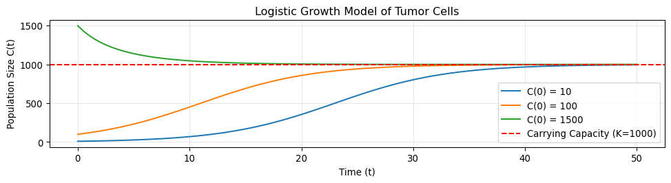
The analytical solution of the logistic growth model is

\[ C(t)=\frac{K}{1+\frac{K-C(0)}{C(0)}e^{-\alpha t}} \]

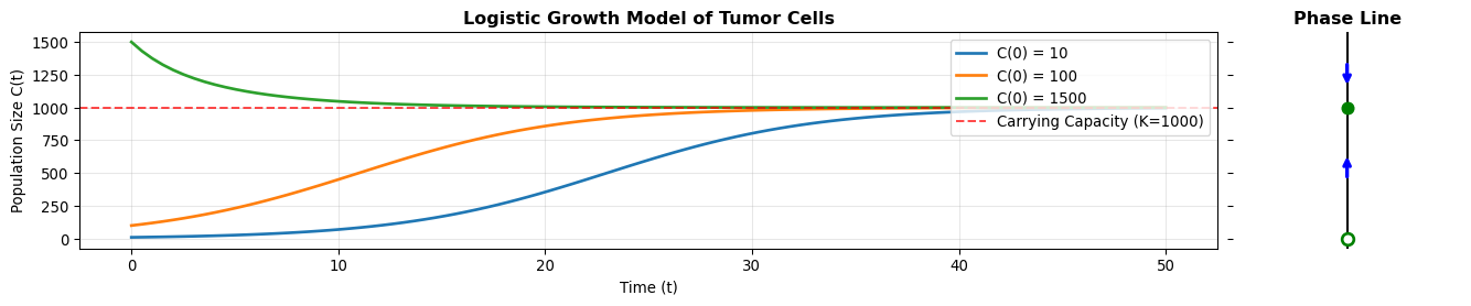
• \(C(t) < K\), the population will grow and reach the carrying capacity \(K\).
• \(C(t) > K\), the population will decline and reach the carrying capacity \(K\).
• \(C(t) = K\), the population will remain constant.

What are missing ?

• The model does not account for interactions with other cell types or the environment.

Consider two populations with following interactions

1. Prey and predator

   • Predator population growth is positively affected by the prey population size
   • Prey population growth is negatively affected by the predator population size

2. Competition between two species

• The growth of each species is negatively affected by the population size of the other species.

\(\rightarrow\) The ODE needs to be modified to account for the interactions between populations.

Lotka-Volterra competition model

Given two species, \(C_1\) and \(C_2\) in competition with each other, the competitive Lotka-Volterra model can be expressed as

\[ \begin{aligned} \frac{dC_1}{dt} = \alpha_1 C_1(t) (1 - \frac{C_1(t) + \beta_{12} C_2(t)}{K_1}) \\ \frac{dC_2}{dt} = \alpha_2 C_2(t) (1 - \frac{C_2(t) + \beta_{21} C_1(t)}{K_2}) \end{aligned} \]

• \(\alpha_1\) and \(\alpha_2\) are the intrinsic growth rates of species 1 and 2, respectively.
• \(K_1\) and \(K_2\) are the carrying capacities of the environment for species 1 and 2, respectively.
• \(\beta_{12}\) and \(\beta_{21}\) are the competition rates between species 1 and 2,
  • \(\beta_{12}\) represents the effect of species 2 on the growth of species 1.
  • \(\beta_{21}\) represents the effect of species 1 on the growth of species 2.

Lotka-Volterra prey-predator model

Given two species, \(C_1\) (prey) and \(C_2\) (predator), the prey-predator Lotka-Volterra model can be expressed as

\[ \begin{aligned} \frac{dC_1}{dt} &= \alpha_1 C_1(t)(1 - \frac{C_1(t)}{K_1}) - \beta_{12} C_1(t) C_2(t) \\ \frac{dC_2}{dt} &= -\alpha_2 C_2(t) + \beta_{21} C_1(t) C_2(t) \end{aligned} \]

• \(\alpha_1\) is the intrinsic growth rate of the prey population
• \(\alpha_2\) is the intrinsic death rate of the predator population in the absence of prey.
• \(\beta_{12}\) is the effect of the presence of predators on the prey death rate.
• \(\beta_{21}\) is the effect of the presence of prey on the predator’s growth rate.

Evaluating system of Ordinary Differential Equations (ODEs)

Qualitative inspection on ODEs

• Systems of ODEs rarely have analytical solutions.
• In many cases where ODEs do not have analytical solutions, we can use qualitative inspection to understand the behavior of the system.
• Phase diagram: Plotting derivatives as an arrow field, which can provide insights into the stability and behavior of the system at given points.

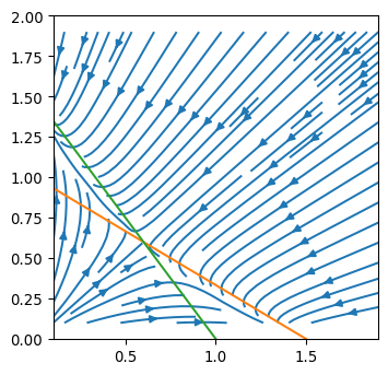
2D Phase diagram

• For a linear ODE system \[ \frac{d\vec{x}}{dt} = A \vec{x} \]

There are three types of equilibrium points:

• Node:

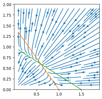
Discussion on Lotka-Volterra competition model

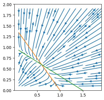
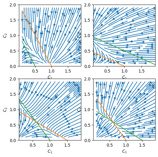
We can find the equilibrium points of the system by setting \(\frac{dC_1}{dt} = 0\) and \(\frac{dC_2}{dt} = 0\), which gives us the following equations:

\[ \begin{aligned} C_1(t) &= K_1 - \beta_{12} C_2(t) \\ C_2(t) &= K_2 - \beta_{21} C_1(t) \\ \end{aligned} \]

The intersection of these lines represents the equilibrium points of the system. (Detailed discussion can be found in McGehee and Mori (2024))

Exclusion of one species (\(C_1\) or \(C_2\) wins)

\(C_1\) wins

• Condition: \(\beta_{12} < \frac{K_1}{K_2}\) and \(\beta_{21} > \frac{K_2}{K_1}\)
• Mechanism: Species 1 exerts strong competitive pressure on Species 2 (\(\beta_{21}\) is large), while Species 2 exerts weak pressure on Species 1 (\(\beta_{12}\) is small).
• Equilibria:
  • \((K_1, 0)\) is a globally stable node.
  • \((0, K_2)\) is an unstable node.
  • \((0, 0)\) is an unstable saddle.

\(C_2\) wins

• Condition: \(\beta_{12} > \frac{K_1}{K_2}\) and \(\beta_{21} < \frac{K_2}{K_1}\)
• Mechanism: Species 2 exerts strong competitive pressure on Species 1 (\(\beta_{12}\) is large), whereas Species 1 exerts weak pressure on Species 2 (\(\beta_{21}\) is small).
• Equilibria:
  • \((K_1, 0)\) is an unstable node.
  • \((0, K_2)\) is a globally stable node.
  • \((0, 0)\) is an unstable saddle.

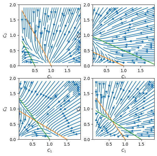
Bistability / Competitive Exclusion

• Condition: \(\beta_{12} > \frac{K_1}{K_2}\) and \(\beta_{21} > \frac{K_2}{K_1}\)
• Mechanism: Interspecific competition is stronger than intraspecific competition for both species. Each species inhibits the other more than it inhibits itself.
• Equilibria:
  • \((K_1, 0)\), \((0, K_2)\) are locally stable nodes.
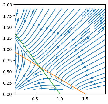
  • The interior intersection point \((C_1^*, C_2^*)\) exists but is a saddle point (unstable): \[C_1^* = \frac{K_1 - \beta_{12}K_2}{1 - \beta_{12}\beta_{21}}, \quad C_2^* = \frac{K_2 - \beta_{21}K_1}{1 - \beta_{12}\beta_{21}}\]
• Outcome: Priority Effect / Founders’ Advantage. The surviving species depends strictly on the initial condition relative to the stable manifold of the saddle point.

Stable Coexistence

• Condition: Condition: \(\beta_{12} < \frac{K_1}{K_2}\) and \(\beta_{21} < \frac{K_2}{K_1}\)
• Mechanism: Intraspecific competition is stronger than interspecific competition for both species. Each population limits its own growth more than it limits the growth of its competitor.
• Equilibria:
  • \((K_1, 0)\), \((0, K_2)\) are unstable nodes.
  • The interior intersection point \((C_1^*, C_2^*)\) is a globally stable node.
• Outcome: Both species coexist indefinitely at reduced population levels relative to their single-species carrying capacities.

Solving ODEs in computer

Preface

Before we really go into the modeling, we need to understand how to solve ordinary differential equations (ODEs) in computer.

In mathematics

• ODEs can be solved analytically (e.g., separation of variables, integrating factor, etc.)
• If ODE does not have an analytical solution, mathematical techniques can be used to qualitatively analyze the behavior of the system (e.g., phase diagram, stability analysis, etc.)

In computer

• ODEs can be solved numerically (Computer can only perform a finite number of calculations, so we need to approximate the solution at discrete time steps)
• Numerical methods can be used to solve ODEs that do not have an analytical solution, or to simulate the behavior of a system over time.

The Initial Value Problem (IVP)

We aim to solve an ordinary differential equation (ODE) of the form:

\[\frac{dy}{dt} = f(t, y), \quad y(t_0) = y_0\]

• Analytical solutions are sometimes difficult or impossible to find for non-linear systems
• Numerical methods approximate the solution at discrete time steps: \[t_0, t_1, t_2, \dots, t_n, t_{n+1}\]
• Where \(h = t_{n+1} - t_n\) represents the step size.
• Again, the computer can only perform a finite number of calculations, in any case computing the solution at discrete time steps is necessary.

Overview of Numerical Integration

The fundamental problem is to evaluate the integral over a single time step:

\[y(t_{n+1}) = y(t_n) + \int_{t_n}^{t_{n+1}} f(t, y(t)) \, dt\]

Numerical integration methods approximate the area under the curve \(f(t, y(t))\) using different strategies:

Where

\[ \frac{dy}{dt} = f(t, y(t)) \]

Intuitively, we can think of \(f(t, y(t))\) as the slope of the solution curve at time \(t\). The integral represents the total change in \(y\) over the interval from \(t_n\) to \(t_{n+1}\).

Evaluating different methods of numerical integration

Imaging we are doing a integration like Reimann sum. In Reimann sum we assume \(dt\) is small enough to accurately approximate the area under the curve. In numeric integration, we need to consider how good is it.

• Stability Error is bound and does not grow exponentially with time steps. Important for long-term simulations. (As an analogy in statistics, we want to make sure the estimator is consistent)
• Accuracy The numerical methods should be close to the true solution.
• Computational cost The method should be computationally efficient, especially for large systems or long simulations.

The Simplest Method: Euler’s Forward Method

By approximating the derivative with a forward finite difference:

\[\frac{y_{n+1} - y_n}{h} \approx f(t_n, y_n)\]

We obtain the explicit Euler update rule:

\[y_{n+1} = y_n + h \cdot f(t_n, y_n)\]

Limitations

• Demands very small \(h\) to avoid numerical divergence in dynamic systems.
• Local Truncation Error (LTE): \(\mathcal{O}(h^2)\)
• Global Truncation Error (GTE): \(\mathcal{O}(h)\) (First-order accurate)

Runge-Kutta (RK) Methods

• Core Idea: Instead of evaluating the derivative only at the beginning of the interval (\(t_n\)), evaluate \(f(t,y)\) at several carefully chosen intermediate trial points within \([t_n, t_{n+1}]\).
• A weighted average of these intermediate slopes is used to compute the final step update.
• Naming convention: \(RKX\) denotes a Runge-Kutta method that evaluates \(f(t,y)\) at \(X\) intermediate points.
• e.g. Euler’s Method is simply a first-order Runge-Kutta method (\(RK1\)).

Developed around 1900 by Carl Runge and Martin Kutta, this family of methods improves accuracy without requiring higher-order derivatives of \(f(t,y)\).

The Classic RK4 Method

The most widely used explicit RK method balances computational cost and high accuracy. To step from \(y_n\) to \(y_{n+1}\), calculate four intermediate slopes:

\[\begin{aligned} k_1 &= f(t_n, y_n) \\ k_2 &= f\left(t_n + \frac{h}{2}, y_n + h\frac{k_1}{2}\right) \\ k_3 &= f\left(t_n + \frac{h}{2}, y_n + h\frac{k_2}{2}\right) \\ k_4 &= f(t_n + h, y_n + h k_3) \end{aligned}\]

Once the four slopes are computed, the next value is calculated via a weighted average resembling Simpson’s Rule:

\[y_{n+1} = y_n + \frac{h}{6} \left(k_1 + 2k_2 + 2k_3 + k_4\right)\]

The RK4 Update Rule

Geometric Intuition

• \(k_1\) is the slope at the left boundary.
• \(k_2\) and \(k_3\) are trial slopes at the midpoint.
• \(k_4\) is a trial slope at the right boundary.

Error Properties

• LTE: \(\mathcal{O}(h^5)\)
• GTE: \(\mathcal{O}(h^4)\)
• Order: \(4^{\text{th}}\)-Order accurate.

Summary and Comparison

Table: Comparison of Fundamental Numerical Integration Methods

Method	Type	Global Error (GTE)	Evaluations per Step	Ideal Use Case
Forward Euler	Explicit	\(\mathcal{O}(h)\)	1	Quick prototyping, highly linear models
Backward Euler	Implicit	\(\mathcal{O}(h)\)	1 (plus solver)	Stiff equations, absolute stability
RK2 (Heun’s)	Explicit	\(\mathcal{O}(h^2)\)	2	Moderate accuracy balance
RK4	Explicit	\(\mathcal{O}(h^4)\)	4	General purpose, non-stiff dynamic systems

Explicit vs Implicit Methods

Explicit Methods

Evaluate \(f(t,y)\) at known, previous time steps. Easy to compute but require small step sizes for stability.

Implicit Methods

Evaluate \(f(t,y)\) involving the unknown future state \(y_{n+1}\). Computationally intensive but highly stable for stiff equations.

Bibilography notes

Bruchovsky, Nicholas, Laurence Klotz, Juanita Crook, Shawn Malone, Charles Ludgate, W James Morris, Martin E Gleave, and S Larry Goldenberg. 2006. “Final Results of the Canadian Prospective Phase II Trial of Intermittent Androgen Suppression for Men in Biochemical Recurrence After Radiotherapy for Locally Advanced Prostate Cancer: Clinical Parameters.” Cancer 107 (2): 389–95.

Greaves, Mel, and Carlo C Maley. 2012. “Clonal Evolution in Cancer.” Nature 481 (7381): 306–13.

McGehee, Cordelia, and Yoichiro Mori. 2024. “A Mathematical Framework for Comparison of Intermittent Versus Continuous Adaptive Chemotherapy Dosing in Cancer.” Npj Systems Biology and Applications 10 (1): 140.

Perera, Marlon, Matthew J Roberts, Laurence Klotz, Celestia S Higano, Nathan Papa, Shomik Sengupta, Damien Bolton, and Nathan Lawrentschuk. 2020. “Intermittent Versus Continuous Androgen Deprivation Therapy for Advanced Prostate Cancer.” Nature Reviews Urology 17 (8): 469–81.

Walsh, Christopher A. n.d. “Accurate Single-Cell Genomic Analysis Holds the Key to Understanding Cancer Heterogeneity.”