Interrupted Time Series Analysis

with SPSS and R example

Yu Cheng Hsu

Learning objectives

• Perform Interrupted Time Series Analysis
• Interpret the results of Interrupted Time Series Analysis

Overview and Intuition

Interrupted Time Series (ITS)

• Study design: Quasi-experimental evaluation design
• Goal: Determine intervention led to a statistically significant change in an outcome.

The Statistical Model

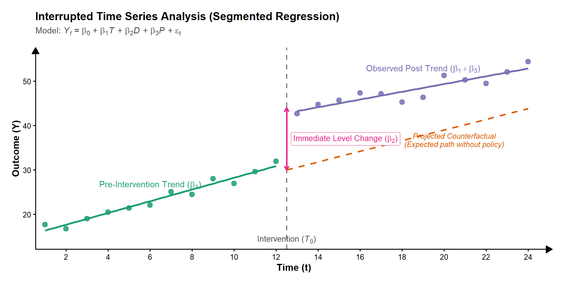
The standard segmented regression equation fitted in SPSS is:

\[ Y_t = \beta_0 + \beta_1 T_t + \beta_2 D_t + \beta_3 P_t + \epsilon_t \]

Variable Name	Coding Rule	Meaning
Time (\(T_t\)) Continuous Time	\(1, 2, 3, \dots, N\)	Baseline pre-intervention slope per time unit (\(\beta_1\)).
Intervention (\(D_t\)) Level Shift	\(0\) before intervention; \(1\) after intervention	Immediate vertical jump or drop right after the policy begins (\(\beta_2\)).
Time_Post (\(P_t\)) Trend Shift	\(0\) before intervention; \(1, 2, 3, \dots\) after intervention	Difference between pre- and post-intervention slopes (\(\beta_3\)).

ITS compares the

• observed post-intervention trajectory against a
• projected counterfactual trajectory (what would have happened if the pre-intervention trend had simply continued unchanged).

IF an internvetion does not work at all.

• \(\beta_2 = 0\): The intervention does not have immediate effect on the observation
• \(\beta_3 = 0\): The intervention does not change the growth rate of the observation