Introduction to R

Ecosystem, Variables, and Operations

Yu Cheng Hsu

About me

• My background:
  • Applied statistician
  • Data scientist
• My research focus
  • Population mental health
  • Text-based counseling
• Office hour: By appointment

AI-policy

• Large language models (LLMs) perform well in answering most programming questions.
• LLMs could potentially help you finish your assignments.
• Their comments can sometimes be inspiring.
• Using LLMs can assist your learning and research.

Core competency in the AI era

• Understand how R works
• Evaluate the outputs from AI
• Articulate the question to instruct AI

R ecosystem

R files

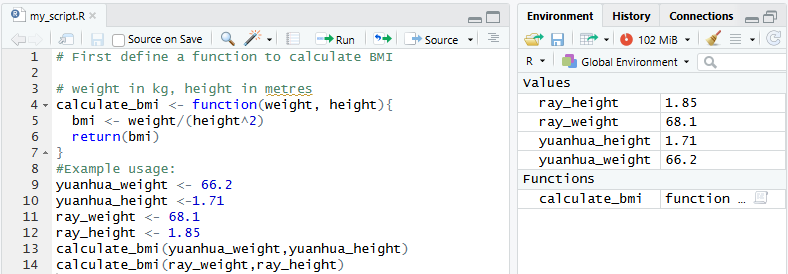
R code can be saved in a text file with the extension .R. You can then run the code in the R console or RStudio by sourcing the file using the source() function. For example, if you have a file named my_script.R, run it with source("my_script.R") in the R console.

Illustration of my_script.R in RStudio

Rmd/QMD files

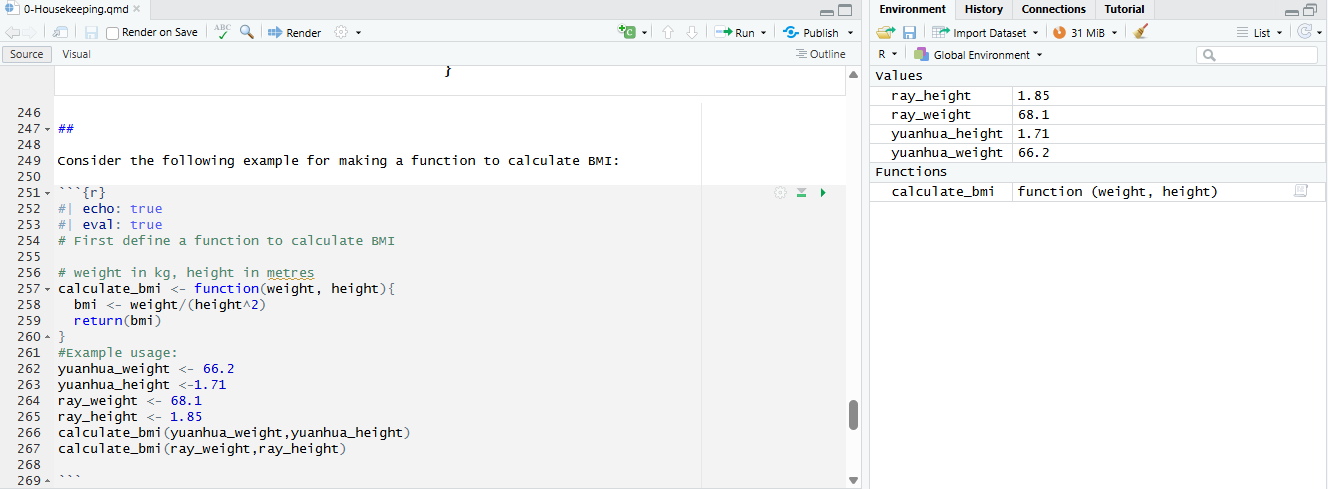
You can save your R code in a file with the extension .Rmd or .qmd. This allows you to create dynamic documents that combine R code, text, and output. For example, the presentation slides are made from an improved version of .qmd.

Illustration of lecture slide (.qmd) in RStudio

RData files

You may save your data or functions to an .RData file and load it with load("PATH/TO/THE/DATA_FILE.RData").

• RStudio may save your last working session, which can sometimes cause trouble.
• The file path can be relative to the current working directory or an absolute path.

Pro tips

• Always clean up your environment while starting new works

Fuoundation of R

Introduction to R

R is a programming language popular for statistical computing, elegant graphics, and genomic data analysis.

Features

• Free and open-source software
• Easy to get started for scientific computing

Slide conventions

• Use code formatting for special terms and examples, such as This or This are code.

# This is a code chunk

Arithmetic operations

R provides many arithmetic and statistical operations like +, -, *, /, %%, and ^

# example of basic operation
2+2

[1] 4

5*3

[1] 15

10/3

[1] 3.333333

10%%3 # %% returns the remainder of the division

[1] 1

2^3 # ^ is the power operation

[1] 8

Variables

Variables store information. To save a value, assign it to a variable. The assignment operator in R is <-. Occasionally, you may also see = used for assignment, but <- is the preferred style in R.

\[ \small \text{Variable <- Value} \]

Benefits of using variables:

• Store and manipulate data in a flexible way.
• Make code more readable and maintainable.
• Allow dynamic programming and automation.

# example of assigning variable called age

age <- 18
age

[1] 18

name <- "John"
name

[1] "John"

Naming conventions for variables

Variables can be called just about anything, but there are some rules in R:

• Special characters like $, #, %, or spaces are not allowed.
• A variable name must start with a letter or a dot (.), but if it starts with a dot, the next character cannot be a digit.
• Variable names are case-sensitive (e.g., age, Age, and AGE are different variables).
• You cannot use particular keywords such as TRUE, FALSE, if, else, or function as variable names as they are reserved for other purposes in R.

Data types

Variables can store different types of data, and R has several built-in data types to support them. The data type of a variable determines what kind of values it can hold and what operations can be performed on it.

You can use the class() and typeof() functions to check the class and data type of any variable. R has five common data types:

1. Numeric
2. Integer
3. Complex
4. Logical
5. Character

Numeric (double)

The numeric data type is for numbers.

• Can be whole numbers or decimals.
• The default numeric type in R.
• Stores values in double precision, so typeof() reports double.

# example of numeric type

height <- 1.70
height

[1] 1.7

class(height)

[1] "numeric"

typeof(height)

[1] "double"

Integer

The integer data type stores whole numbers.

• Use the capital L suffix to create an integer value.
• Convert a numeric value to integer using as.integer().
• Convert an integer to numeric using as.numeric().

# example of integer type

siblings <- 2L
siblings 

[1] 2

typeof(siblings)

[1] "integer"

siblings <- as.numeric(siblings)
typeof(siblings)

[1] "double"

Logical

In R, the logical data type can be:

• TRUE (carries a value of 1)
• FALSE (carries a value of 0)

Tips: Logical values can behave like numbers. Numeric operations are possible on logical values, but use caution.

# example of logic type

male <- TRUE
male

[1] TRUE

typeof(male)

[1] "logical"

male <- male-1
male

[1] 0

typeof(male)

[1] "double"

Character

The character data type stores text strings, including letters, numbers, and symbols. Strings in R can be written with single or double quotes.

# example of character type

name <- "Ray"
name

[1] "Ray"

typeof(name)

[1] "character"

age <- "25"
age

[1] "25"

typeof(age)

[1] "character"

Comparison operations

Comparison operators compare two values and return a logical value TRUE or FALSE.

# example of basic operations
2 == 2 # Equal

[1] TRUE

5 < 3 # Less than

[1] FALSE

10 >= 3 # Greater than or equal to

[1] TRUE

10 != 3 # Not equal

[1] TRUE

## Weird behavior !!
1 == "1"

[1] TRUE

1 == TRUE

[1] TRUE

"1" == TRUE

[1] FALSE

Coercion

while performing any operations mixed with different data types in R, the values are automatically converted to the most general data type by coercion. The order is as below

\[ \text{logical} < \text{integer} < \text{numeric} < \text{character} \]

1.2 + TRUE

[1] 2.2

# 2.3 + "1" <= This line will result in error
## Weird behavior !!
1 == "1"

[1] TRUE

1 == TRUE

[1] TRUE

"1" == TRUE

[1] FALSE

Functions

Functions are used to perform tasks on input values. For example, the sin() function calculates the sine of a number. The input to the function is given inside the parentheses.

\[ \sin (\pi) = 0 \]

# example of sin() function
sin(pi)

[1] 1.224606e-16

• sin is the name of the function, and pi is the input. The output of the function is 0.
• Why is the output not exactly 0? This is because π is stored as a double and is accurate to about 15–16 decimal places. As a result, sin(pi) is a very small number close to zero, but not exactly zero.

More function examples

Another example is floor(), which rounds a number down to the nearest whole number.

# example of floor(sin(pi)) function
sin_pi <- sin(pi)
floor(sin_pi)

[1] 0

• The output of floor(sin(pi)) is 0. This is because the floor() function rounds down the value of sin(pi) to the nearest whole number.
• R has many predefined functions, and you can also create your own functions. See the official documentation for more information.
• Within RStudio, you can use ? to get help on a function. For example, ?floor gives information about the floor() function.

Writing your own function

You can customize functions in R to perform specific tasks. Benefits of using functions:

• Make your code more organized and readable.
• Allow for code reusability and modularity.

The format for writing a function in R is:

\[ \begin{aligned} \textit{function_name} &\leftarrow \text{function}(\textit{arguments}) \{ \\ & \textit{your code} \\ & \} \end{aligned} \]

BMI example

Consider the following example of a function that calculates BMI:

# First define a function to calculate BMI

# weight in kg, height in meters
calculate_bmi <- function(weight, height) {
  bmi <- weight / (height^2)
  return(bmi)
}
# Example usage:
yuanhua_weight <- 66.2
yuanhua_height <- 1.71
ray_weight <- 68.1
ray_height <- 1.85
calculate_bmi(yuanhua_weight, yuanhua_height)

[1] 22.63944

calculate_bmi(ray_weight, ray_height)

[1] 19.89774

Data structures

Data structures are one of the most important features in programming.

• Organize data
• Store data

Benefits - Easier to read - Fasten calculation

Main data structures used in R:

• Vector: A list of items of the same data type, like a series of numbers (numeric) or words (characters).

• Matrix: Tables of numbers with rows and columns, where all elements are the same type.

• List: Collections that can hold different types of data all together, such as numbers, words, or even other lists.

• Data Frame: Like a spreadsheet where each column can have different types of data, useful for tabular data

Vector

• Basic data structure in R.
• Store elements in the same data type.
• Check the data type by using typeof() function
• Check the length of the vector by length() function.
• Coersion will be performed if different data type occurs

# vector of numerics
# c combines numbers in the brackets to a vector
age <- c(16, 20, 15, 17, 18) 
age

[1] 16 20 15 17 18

typeof (age)

[1] "double"

length(age)

[1] 5

See more introduction here.

There are also different ways to automatically generate vectors

Other examples

There are also different ways to automatically generate vectors

# vectors can be created using existing variables
jason <- 1.69
ray <- 1.78
yuanhua <- 1.72

heights <- c(jason, ray, yuanhua)
# you can give names to items in a vector
names(heights) <- c("Jason","Ray","Yuanhua")
heights

  Jason     Ray Yuanhua 
   1.69    1.78    1.72 

typeof(heights)

[1] "double"

# rep repeats the first number
# n times based on the second value
repeats <- rep(3, 5)  
repeats

[1] 3 3 3 3 3

typeof(repeats)

[1] "double"

# generates a vector of integers 
# from 1 to 12 (inclusive)
series <- 1:12 
series

 [1]  1  2  3  4  5  6  7  8  9 10 11 12

typeof(series)

[1] "integer"

# generate a vector of random integers by sampling
# 6 values between 1 and 49 (六合彩)
mark6 <- sample(1:49,6)
mark6

[1] 32 49  8 29 47  4

typeof(mark6)

[1] "integer"

Combining vectors

Vectors can also be combined from other vectors.

# vectors can be combined
new_vector <- c(series,mark6,rep(50,3))
new_vector

 [1]  1  2  3  4  5  6  7  8  9 10 11 12 32 49  8 29 47  4 50 50 50

typeof(new_vector)

[1] "double"

Did you notice that new_vector is now a of type double ?

You can spend a few minutes to create vectors and explore what happens to the data type of the vector when you combine them with others.

# write your code here
myVector <- c(TRUE,2:3,4.0)
myVector

[1] 1 2 3 4

typeof(myVector)

[1] "double"

Index

Items in a vector can be directly retrieved by their index

# Example of using index to retrieve items in a vector
scores <- c(44,56,63,75,77,78,81,90,93,99)
scores

 [1] 44 56 63 75 77 78 81 90 93 99

typeof(scores)

[1] "double"

scores[5]              # retrieve score at index 5 (i.e. 5th position) 

[1] 77

scores[2:5]            # retrieve score from index 2 to 5

[1] 56 63 75 77

scores[c(2,5,7)]       # retrieve scores from index 2, 5 and 7

[1] 56 77 81

scores[-5]             # retrieve all scores except index 5

[1] 44 56 63 75 78 81 90 93 99

scores[c(TRUE,FALSE)]  # retrieve scores in odd positions

[1] 44 63 77 81 93

Exercise

Can you write the code to retrieve the scores from:

scores <- c(44,56,63,75,77,78,81,90,93,99)

1. the first position

# write the code to retieve the 1st position
scores[1]

[1] 44

2. even positions

# write the code to retrieve even positions
scores[c(FALSE,TRUE)]

[1] 56 75 78 90 99

3. every 3rd position

# write the code to retrieve every 3rd position
scores[c(FALSE,FALSE,TRUE)]

[1] 63 78 93

Modifying a vector

Using the index it is possible to modify specific items in a vector

# example modifying items in a vector
scores <- c(44,56,63,75,77,78,81,90,93,99)
scores

 [1] 44 56 63 75 77 78 81 90 93 99

# modify position 5
scores[5] <- 50
scores

 [1] 44 56 63 75 50 78 81 90 93 99

# modify positions 1 to 4
scores[1:4] <- c(30,40,50,60)
scores

 [1] 30 40 50 60 50 78 81 90 93 99

# modify position 1 and changes vector to character
scores[1] <- "Twenty"
scores

 [1] "Twenty" "40"     "50"     "60"     "50"     "78"     "81"     "90"    
 [9] "93"     "99"    

Matrix

• Two-dimensional data structure.
• You can think of 2D version of vector
• It has rows and columns, both of which can also have names.
• To check the dimensions, you can use the dim() function.

See more introduction here.

myMatrix <- matrix(1:12, nrow=3)
colnames(myMatrix) <- c("C1","C2","C3","C4")    # assign column names
rownames(myMatrix) <- c("R1","R2","R3")         # assign row names
myMatrix

   C1 C2 C3 C4
R1  1  4  7 10
R2  2  5  8 11
R3  3  6  9 12

dim(myMatrix)                                   # prints dimension of the matrix 

[1] 3 4

Indexing a matrix

Accessing items in a matrix is similar to vector but in 2 dimensions

myMatrix[1, 2]                          # retrieve item in row 1 column 2

[1] 4

myMatrix["R2", "C2"]                    # retrieve item by row and col name in R2, C2

[1] 5

myMatrix[1, 1:2]                        # retrieve items in row 1 and col 1 and 2. 

C1 C2 
 1  4 

myMatrix[1:2, c(2, 3)]                  # retrieve items in row 1-2 and col 2-3

   C2 C3
R1  4  7
R2  5  8

Modify values

Modifying items in a matrix is similar to vector but in 2 dimensions. Can you write the code to:

1. replace row 3, column 3 with the value 7?

myMatrix[3,3] <- 7
myMatrix

   C1 C2 C3 C4
R1  1  4  7 10
R2  2  5  8 11
R3  3  6  7 12

2. replace row 1, column 4 using the row and col name with the value -5?

myMatrix["R1","C4"] <- -5
myMatrix

   C1 C2 C3 C4
R1  1  4  7 -5
R2  2  5  8 11
R3  3  6  7 12

3. delete row 2

myMatrix <- myMatrix[-2, ]
myMatrix

   C1 C2 C3 C4
R1  1  4  7 -5
R3  3  6  7 12

List

• Capable to hold mixed data types. A list can contain a list of any data structure: value, vector, matrix, list, etc.

myList <- list(1.70, TRUE, 1:3, "Ray",list(8,8,4))
str(myList)

List of 5
 $ : num 1.7
 $ : logi TRUE
 $ : int [1:3] 1 2 3
 $ : chr "Ray"
 $ :List of 3
  ..$ : num 8
  ..$ : num 8
  ..$ : num 4

We can use str() function to view the structure of a list (or any object).

names(myList) <- c("Height","Male","Workdays","Name","hour")    # give names to elements in list
str(myList)

List of 5
 $ Height  : num 1.7
 $ Male    : logi TRUE
 $ Workdays: int [1:3] 1 2 3
 $ Name    : chr "Ray"
 $ hour    :List of 3
  ..$ : num 8
  ..$ : num 8
  ..$ : num 4

Indexing list

• double-layer square brackets, either by numeric index or name.
• $ symbol with the name.

# example of retrieving items from a list
myList[[4]] # using index

[1] "Ray"

myList[["Name"]]  # using index of Name

[1] "Ray"

myList$Name # using the Name key directly

[1] "Ray"

Can you retrieve the Height and Name from myList?

myList[c(1,4)] 

$Height
[1] 1.7

$Name
[1] "Ray"

note that unlike the above, the retrieved values are still in a list as opposed to individual values like what you get with double brackets [[]]

myList[c("Height","Name")]

$Height
[1] 1.7

$Name
[1] "Ray"

Converting to/from vector

It is possible to inter-convert list to and from vectors.

# example of interconverting list to vector and back
myList <- list(1.70, TRUE, 1:3, "Jason")
str(myList)

List of 4
 $ : num 1.7
 $ : logi TRUE
 $ : int [1:3] 1 2 3
 $ : chr "Jason"

myVector <- unlist(myList)
myVector

[1] "1.7"   "TRUE"  "1"     "2"     "3"     "Jason"

myList_cov <- as.list(myVector)
str(myList_cov)

List of 6
 $ : chr "1.7"
 $ : chr "TRUE"
 $ : chr "1"
 $ : chr "2"
 $ : chr "3"
 $ : chr "Jason"

Data Frame

Data frame is widely used for rectangular data, where each column has the same data type (vector) but different columns can have different data types (like Excel)

The data frame is in fact a special type of list: A list of vectors with the same length.

myDF <- data.frame("Height" = c(1.70, 1.80, 1.68, 1.72), 
                  "Weight" = c(67, 60, 55, 58), 
                  "Name" = c("Jason", "Ray", "Dora", "Yuanhua"), 
                  "Gender" = factor(c("male","male","female","male")))
myDF

  Height Weight    Name Gender
1   1.70     67   Jason   male
2   1.80     60     Ray   male
3   1.68     55    Dora female
4   1.72     58 Yuanhua   male

myDF$Name[3]          # print name at index 3

[1] "Dora"

levels(myDF$Gender)   # print levels of gender (which is coded as a factor)

[1] "female" "male"  

Comparison

Operator	Description	Example	Returns
==	Equal to	5 == 5	TRUE
!=	Not equal to	5 != 7	TRUE
>	Greater than	10 > 8	TRUE
<	Less than	2 < 4	TRUE
>=	Greater than or equal to	5 >= 5	TRUE
<=	Less than or equal to	3 <= 5	TRUE

Logical operators

Logic operators are used for operating on logic data type (i.e. TRUE or FALSE). The three logical operators are:

• AND &
• OR |
• NOT !

# To test if Ray will have to lecture on Zoom
zoomClass <- function(blackRain, Typhoon8){
  return (blackRain | Typhoon8)
}

zoomClass(TRUE, TRUE) # It is Black Rain and Typhoon 8

[1] TRUE

zoomClass(FALSE, TRUE) # It is only Typhoon 8

[1] TRUE

zoomClass(TRUE, FALSE) # It is only Black Rain

[1] TRUE

zoomClass(FALSE, FALSE) # It is neither

[1] FALSE

If/else

Link logical outcome to an action given the condition. This is where the if and else statement comes in. The format is like

if (CONDITIION) {
  # If CONDITIION==TRUE: codes inside this bracket will be executed
} else {
 # If CONDITIION==FALSE: codes inside this bracket will be executed (You can akso omit this part if needed)
}

Example

# example of if/else based on passing exam
zoomClass <- function(blackRain, Typhoon8){
  if  (blackRain | Typhoon8) {
    print("Zoom link:XXXX")
  }else{
    print("We will have offline class")
  }

}
zoomClass(TRUE, TRUE)

[1] "Zoom link:XXXX"

zoomClass(FALSE, FALSE)

[1] "We will have offline class"

Chained conditions

It is also possible to chain if/else statements if there are multiple conditions:

# example of multiple if else conditions
ageCategory <- function(age){
  if (age <= 12){
    print("Child")
  } else if (age > 12 & age <= 19){
    print("Teenage")
  } else if (age > 20 & age <= 60) {
    print("Adult")
  } else {                                # > 60
    print("Elderly")
  }                              
}

ageCategory(5)

[1] "Child"

ageCategory(45)

[1] "Adult"

ageCategory(70)

[1] "Elderly"

Loop

• Using loop to reduce redundant code

Here are some simple examples of a for loop in R:

# examples of loop
# Loop printing a series of numbers from 1 to 10
for (i in 1:10){
  print(i)
}

[1] 1
[1] 2
[1] 3
[1] 4
[1] 5
[1] 6
[1] 7
[1] 8
[1] 9
[1] 10

You can also iterater on vectors

# Loop printing a vector of names
names <- c("Jason","Ray","Yuanhua")
for (i in names){
  print(i)
}

[1] "Jason"
[1] "Ray"
[1] "Yuanhua"

Survival Guide: R Debugging & AI Assistance

Preface

• You will encounter errors.
• Getting an error in R is not a sign of failure;
• it is simply R’s way of asking for clarification, or
• The program is not desgined to work in that way

Part 1: How to Read the Red Text Without Panicking

When R throws red text at you, first determine what kind of message it is:

1. Message / Note: Just R talking to you (e.g., “The tidyverse packages have been loaded”). Action: Ignore.
2. Warning: The code did run, but something looks suspicious to R (e.g., Removed 5 rows containing missing values). Action: Read it, verify if it affects your analysis, but no immediate panic.
3. Error: The code stopped. R cannot proceed. Action: Time to debug.

Identifying the key of the Error

Don’t read the whole error if it looks messsy. Look for the recognizable words at the end of the message.

Common Biomedical Data Errors translated to plain English:

• Error: object 'XXX' not found
  • Translation: You either haven’t run the line of code that creates/loads XXX yet, or you made a typo (e.g., you typed xxx).
• Error in read_csv("FILE") : could not find function "read_csv"
  • Key: could not find function
  • Translation: You forgot to load the package! Run library(tidyverse) or library(readr) first.
• Error: unexpected symbol in "ggplot(data = clinical_df aes(x = treatment))"
  • Key: unexpected symbol
  • Translation: You missed a comma. (There should be a comma after clinical_df).

Part 2: The AI Lifeline

When the error is confusing, Large Language Models (LLMs) are your best teaching assistants. However, “Garbage In = Garbage Out.”

Bad example

My R code doesn’t work!!!!!

Asking right question

To get an immediate, accurate fix, always provide the AI with these three components:

1. The Goal: What you are trying to do (briefly).
2. The Code: The exact lines that failed.
3. The Error: The exact copy-pasted red text.

Copy-Paste Prompt Template:

Act as an expert R programmer

Goal: I am trying to [e.g., create a scatterplot of gene expression versus patient age using ggplot2].

Here is my code:

[Paste your code here]

Here is the error message I received:

[Paste the EXACT error message here]

Please tell me what went wrong and provide the corrected code.

Part 3: Best Practices for AI-Assisted Coding

1. Don’t just copy-paste the fix: Always read the AI’s explanation. If you just copy-paste, you will make the exact same error tomorrow. Ask yourself: “What was the key of my mistake?”
2. Watch out for Hallucinations: AI sometimes invents R functions that don’t exist. If the AI’s code throws a new error saying could not find function..., reply to the AI with that new error!
3. Protect Sensitive Data: NEVER paste real, identifiable patient data or confidential research results into LLM. If the AI asks to see your data structure, use str(your_data) or head(your_data) and mock up the values, or simply provide the column names.

Resource links

This notebook adapts contents from these resources:

• https://www.datamentor.io/r-programming/
• https://www.geeksforgeeks.org/r-data-types/
• https://data-flair.training/blogs/r-data-types/

Special thanks to Prof. Yuanhua Huang, and Prof Jason Wong.