EHR data and linear regression

SBMS7402 — session materials

Yu Cheng Hsu

Intended learning outcomes

By the end of this session, you will be able to:

Explain what an EHR contains and why coding standards matter
Interpret a simple linear model on continuous healthcare-style data
Read one residual diagnostic plot and say what assumption it checks

This week’s path

EHR — what is in the digital chart, and common data traps
Why regression — summarize “how \(y\) changes with \(x\)”
Diagnostics — check whether the line’s assumptions look reasonable

What is an EHR?

An Electronic Health Record (EHR) is the digital chart of a patient’s encounters with the health system—visits, diagnoses, labs, prescriptions, and clinical notes stored so clinicians (and later analysts) can reuse them.

Toy timeline (one patient):

Visit the clinic → demographics recorded
Doctor records a diagnosis → coded (e.g. ICD)
Lab is ordered → result coded (e.g. LOINC)
Prescription is filled → drug coded (e.g. ATC / RxNorm)

Coding systems are a shared language so different hospitals and software can mean the same clinical idea.

Components in EHR System

Demographics & Social Determinants: Age, sex, ethnicity, socioeconomic indicators.
Clinical Encounters & Diagnoses: Coded using international diagnostic standards:
- ICD-9 / ICD-10 / ICD-11: International Classification of Diseases.
- SNOMED-CT: Systematized Nomenclature of Medicine for clinical concepts.
Prescriptions & Pharmacy Records: Coded using ATC or RxNorm frameworks.
Laboratory & Diagnostic Results: Coded using LOINC standards.
Unstructured Clinical Text: Progress notes, discharge summaries, radiological reports.

From Individual Care to Population & Global Health

Scaling clinical observations from single patient encounters to entire populations.
Clinical Medicine: Focuses on diagnosis, treatment, and immediate patient outcomes.
Population Health: Health outcomes, determinants, and patterns across defined groups (e.g., regional populations, disease cohorts).
Global Health & Digital Health Venture: Scalable health solutions, cross-border disease surveillance, and commercialization of data-driven digital health products.

EHR for idea generation

Problem

Many biomedical startups fail due to building solutions for undersized or ill-defined patient markets.
How many potential customers could benefit from the product?

EHR can

Analyzing epidemiological EHR data allows founders to precisely quantify unmet clinical needs
Facilitate further pricing strategy, potential market size.

EHR as a product

Problem

Using EHR to develop new algorithms for diagnostic AI
Software-as-a-Medical-Device (SaMD: software that itself is regulated as a medical device)
Enhance accessibility of EHR, e.g. dashboard

EHR can

Provide fruitful training sources
Serve as an information service for clinical decisions

EHR as an evidence

Problem Traditional Randomized Controlled Trials (RCTs) are

expensive,
slow, and often lack generalizability.

EHR can

Regulatory bodies (e.g., US FDA, EMA, NMPA) increasingly accept real-world evidence (RWE)—evidence generated from routine care data such as EHRs, not only from traditional trials—for

Post-market surveillance,
Label expansions, and
Synthetic control arms in clinical trials.

Challenges in EHR

Missingness (missing for a reason)

Clinic vignette: sicker patients get more labs ordered; healthier patients may have blank lab fields. A “missing” lab is often informative, not random noise.
Formal label: this pattern is often called missing not at random (MNAR) (contrast: completely random gaps vs gaps explained by other recorded variables).
Labs/tests are ordered based on clinical suspicion, leading to missing baseline data.
Loss to follow-up due to stigma and/or economic difficulties.

Selection / Sampling Bias

EHRs represent health-seeking populations, not necessarily the general population.
People who are not covered in the health care system

Measurement / Coding Error

Inaccurate ICD codes or changes in institutional coding policies over time.
Human errors in the process
Misdiagnosis

Linear Regression & Diagnostics

Why fit a line? (intuition first)

Healthcare question: Does systolic blood pressure tend to rise with age?

Plot age (\(x\)) against blood pressure (\(y\)): points scatter, but often show an upward trend.
A best-fit line summarizes that trend: “on average, how does \(y\) change as \(x\) increases?”

In plain English

\(\beta_1\): average change in \(y\) for a one-unit increase in \(x\) (holding other predictors fixed, when there are several)
\(\beta_0\): predicted \(y\) when all predictors are zero (often not clinically meaningful; still needed mathematically)
\(\epsilon\): leftover person-to-person noise the line does not explain

We fit the line so we can describe, predict, and later test whether a relationship is compatible with chance.

Introduction to the Linear Regression Model

With that intuition, the linear regression model is formally defined as \[ \begin{aligned} y_{i} = & \beta_{0} + \beta_{1}x_{1i} + \beta_{2}x_{2i} + \dots + \beta_{p}x_{pi} + \epsilon_{i} \text{, or}\\ \mathbb{y} = &\mathbb{\beta}\mathbb{X}+ \mathbb{\epsilon} \end{aligned} \]

Systematic part (predictors / independent variables)
Random part: individual outcomes vary by an error term \(\epsilon_{i}\)
It is assumed that \(\epsilon_{i} \sim \mathcal{N}(0, \sigma_{\epsilon}^{2})\)

Optional / advanced

The matrix form \(\mathbf{y}=\boldsymbol{\beta}\mathbf{X}+\boldsymbol{\epsilon}\) is a compact way to write the same model for many predictors. Focus first on the scalar equation and the meaning of \(\beta\) and \(\epsilon\).

Prediction in regression

Confidence Interval (CI) for the Mean Response: The average expected outcome for all individuals with a specific predictor value \(x\)

Uncertainty: Uncertainty on \(\mathbb{\beta}\)

Prediction Interval (PI) for a New Observation: Predict the specific outcome \(y\) for a single, new individual with a specific predictor value \(x\).

Uncertainty: Uncertainty on \(\mathbb{\beta}\) and Uncertainty on \(\mathbb{X}\)

Evaluating regression

\(y_i\): The actual observed value.
\(\hat{y}_i\): The predicted value on the regression line.
\(\bar{y}\): The mean of all observed \(y\) values.

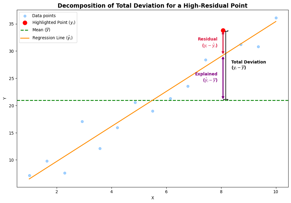
The following relationship holds \[TSS = ESS + RSS\] TSS (Total Sum of Squares): \[\sum (y_i - \bar{y})^2\] ESS (Explained Sum of Squares): \[\sum (\hat{y}_i - \bar{y})^2\] RSS (Residual Sum of Squares):\[\sum (y_i - \hat{y}_i)^2\]

\(R^2\): The Coefficient of Determination

\(R^2\) is the percentage of variance explained by the linear model

\[ R^2 = \frac{ESS}{TSS} = 1 - \frac{RSS}{TSS} \]

\(R^2 = 0\): the model explains none of the variance in the outcome (the regression line is flat at the mean, \(\bar{y}\)).
\(R^2 = 1\): the model explains 100% of the variance (every data point falls exactly on the regression line, meaning RSS is zero).

Inference on linear model

Even if we have \(R^2\), we need to know whether the explained variance is statistically significant.
Null Hypothesis \[ H_0: \beta_1 = \beta_2 = \dots = \beta_p = 0 \]
Test statistics

\[ F = \frac{ESS / df_{ESS}}{RSS / df_{RSS}} \sim F_{df_{ESS},df_{RSS}} \]

\(df_{ESS} = p\) (the number of predictor variables)
\(df_{RSS} = n - (p + 1)\) (the number of observations minus the total number of estimated parameters, including the intercept)

Inference on individual \(\beta_i\)

Investigate whether each predictor makes a statistically significant contribution to the outcome
Null Hypothesis \[ H_0: \beta_i = 0 \]
Test statistics

\[ \beta_i \sim t_{n-(p+1)}(0,\frac{s_{y\vert{}x}^{2}}{(n-1)s_{x_i}^{2}(1-r_{i}^{2})}) \]

Implication in linear model: Including other predictors to control for confounding commonly makes it more difficult to reject the null hypothesis
Some of the unadjusted association is explained by those other predictors.

Assumption on linear regression

Ask these in everyday language first (formal names in parentheses):

Is the trend roughly a straight line? (Linearity)
Do leftovers look roughly bell-shaped? (Normality of errors)
Are leftovers independent (not clustered in time, space, or repeated measures)? (Independence of errors)
Is the leftover scatter similar at low and high fitted values? (Homoscedasticity / constant variance)
Are two predictors saying almost the same thing? (No multicollinearity)

Failure modes matter clinically: e.g. if sicker patients get more labs, associations estimated from complete cases can be biased.

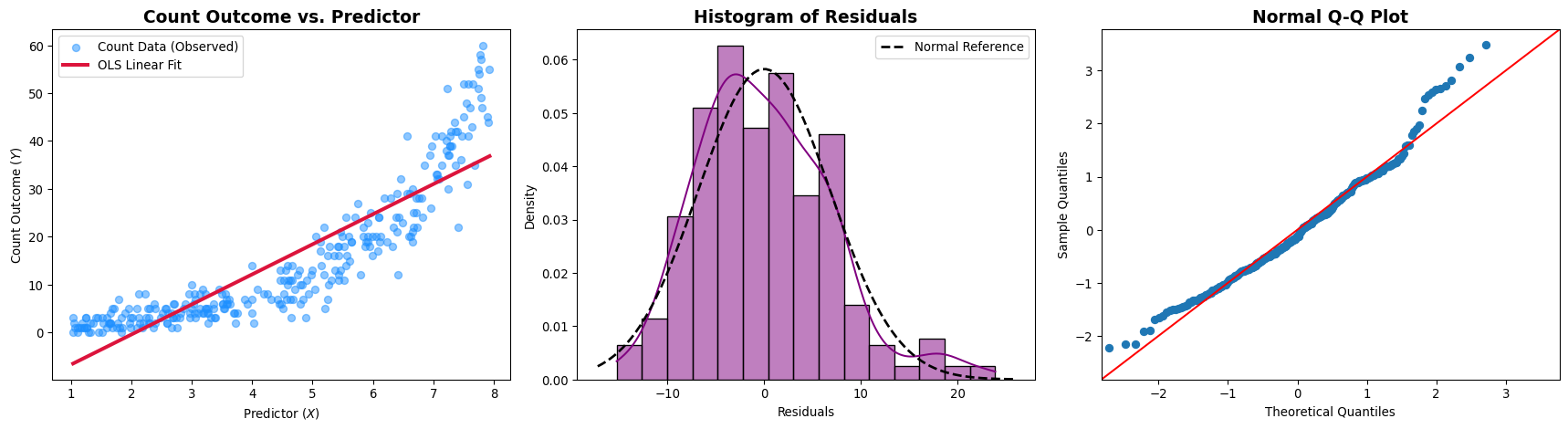
Linearity

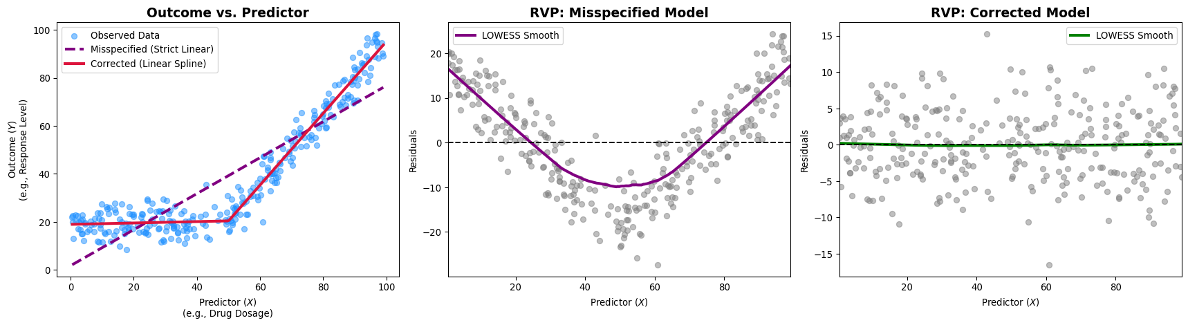
Plain check: Does \(y\) change at a roughly constant rate as \(x\) increases, or is there a bend / threshold?

The model assumes that the outcome changes linearly with each continuous predictor.

Checking:

Residual versus Predictor (RVP) plots

Mitigation plan linearity

Categorize the continuous predictor.

The predictor has the threshold effect
Transformations to the predictor (e.g., adding quadratic terms, log transformations)

The predictor has the non-linear effect on the outcome
Piecewise Regression

Specifying a threshold point in the regression model

Normality of Errors

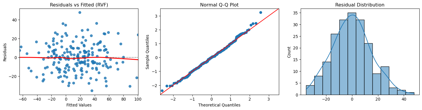
Plain check: Do residuals look like a bell (symmetric pile around zero), or are they piled on one side / heavy-tailed?

\(\epsilon \text{i.i.d} N(0,1)\) is assumed
Normality checking with Q-Q plot:
- Diagonal line: Normal
- Upward curvature: Residuals are right-skewed (Floor effects of X).
- Downward curvature: Residuals are left-skewed (Ceiling effects of X).

Mitigation plan

Transforming the outcome variable (e.g., replacing \(y\) with \(log(y)\))
This could also imply other regression (i.e. Poisson, Negative-binomial regression)

Independence of errors

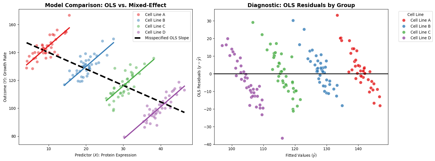
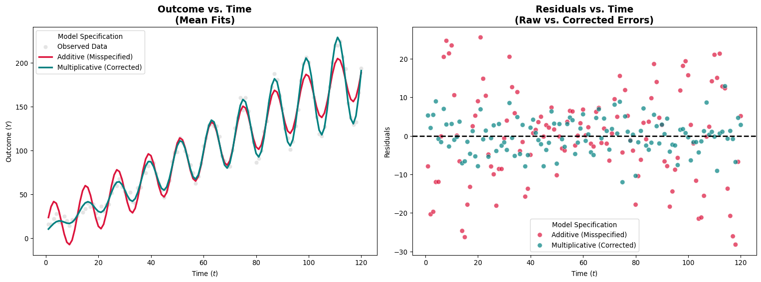
Plain check: Is each leftover “its own story,” or are nearby / same-patient / same-clinic residuals similar?

\(\epsilon \text{ i.i.d} N(0,1)\) is assumed

Some obvious situations that violate this assumption

Repeated measures on the same person
Temporal or spatial patterns among observations

Checking the group difference

Constant Variance (Homoscedasticity)

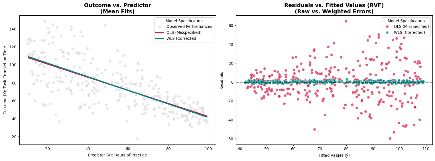
Plain check: Is the leftover scatter similar across the range of fitted values, or does it fan out like a funnel?

Constant variance of the error term, \(\sigma_{\epsilon}^{2}\) (violation = heteroscedasticity)
Impact: Precision of confidence intervals and P-values.
Checking: Residual versus Fitted (RVF) plots.
A horizontal funnel shape in these scatterplots is a signal of heteroscedasticity.
Having more observations won’t relieve the problem

Influential Points and Outliers

High leverage points are x-outliers with the potential to exert undue influence on regression coefficient estimates. Influential points are specific observations that have actually exerted an undue influence on the estimates. DFBETA statistics are recommended to quantify how much each coefficient would change if a specific observation were omitted from the dataset.

Code Illustrations: Python and R

Below are examples of how to fit a multiple linear regression model and generate the necessary diagnostic plots in both Python and R.

Python illustration

                            OLS Regression Results                            
==============================================================================
Dep. Variable:                      Y   R-squared:                       0.810
Model:                            OLS   Adj. R-squared:                  0.808
Method:                 Least Squares   F-statistic:                     420.6
Date:                Thu, 13 Aug 2026   Prob (F-statistic):           7.92e-72
Time:                        16:13:04   Log-Likelihood:                -821.84
No. Observations:                 200   AIC:                             1650.
Df Residuals:                     197   BIC:                             1660.
Df Model:                           2                                         
Covariance Type:            nonrobust                                         
==============================================================================
                 coef    std err          t      P>|t|      [0.025      0.975]
------------------------------------------------------------------------------
const         25.7620      7.528      3.422      0.001      10.917      40.607
X1             2.2881      0.114     20.148      0.000       2.064       2.512
X2            -1.2151      0.054    -22.687      0.000      -1.321      -1.110
==============================================================================
Omnibus:                        1.716   Durbin-Watson:                   1.916
Prob(Omnibus):                  0.424   Jarque-Bera (JB):                1.565
Skew:                           0.217   Prob(JB):                        0.457
Kurtosis:                       3.012   Cond. No.                         822.
==============================================================================

Notes:
[1] Standard Errors assume that the covariance matrix of the errors is correctly specified.

R illustration

# 1. Generate Synthetic Data
set.seed(42)
n <- 200
X1 <- rnorm(n, mean=50, sd=10)
X2 <- rnorm(n, mean=100, sd=20)
# Create outcome with normal noise
Y <- 15 + 2.5*X1 - 1.2*X2 + rnorm(n, mean=0, sd=15)

data <- data.frame(Y, X1, X2)

# 2. Fit the Linear Regression Model
model <- lm(Y ~ X1 + X2, data=data)

# Print model summary (Contains F-test, RSS, and coefficients)
print(summary(model))

# 3. Residual Diagnostics
# R has built-in diagnostic plots that are generated by plotting the model object
par(mfrow=c(2,2)) # Set up a 2x2 grid for plots

# Plot 1: Residuals vs Fitted (checks linearity and constant variance)
# Plot 2: Normal Q-Q (checks normality of residuals)
# Plot 3: Scale-Location (checks homoscedasticity)
# Plot 4: Residuals vs Leverage (checks for influential points / high leverage)
plot(model)