Network science

for social science

Dr. Yu Cheng Hsu

Learning objectives

• Understand basic network science metrics
• Literate and understand probabilstic graphical model
• Literate and understand ergm model

Cover background Mondrian (1942)

Introduction to Network Science

Network Science?

• Definition: An interdisciplinary field studying the topology, dynamics, and interactions of complex systems through graph theory.
• Focuses on organizing principles across diverse domains without requiring advanced pure mathematics or algorithms.

• Foundational Literature:
  • Barabási (2013), Network Science
  • Newman (2018), Networks
  • Menczer, Fortunato, and Davis (2020), A First Course in Network Science

Mathematical Formalism

A network is mathematically defined as a graph \(G = (V, E)\):

• Vertex / Node Set: \(V = \{v_1, v_2, \dots, v_N\}\), where \(|V| = N\) is the network size.
• Edge / Link Set: \(E = \{(u, v) \mid u, v \in V\}\), where \(|E| = M\) is the total edge count.

Notation

In directed graphs, an edge \(e = (u, v)\) points from source \(u\) to target \(v\) (often termed a directed arc).

Adjacency Matrix Representation

A graph \(G\) with \(N\) vertices is represented by an \(N \times N\) adjacency matrix \(A\):

\[ A_{ij} = \begin{cases} 1 & \text{if } (i, j) \in E \\ 0 & \text{otherwise} \end{cases} \]

• Undirected Networks:
  • Symmetric: \(A_{ij} = A_{ji}\)
  • Reciprocal interaction
• Directed Networks:
  • Asymmetric: \(A_{ij} \neq A_{ji}\)
  • \(A_{ij} = 1 \implies i \to j\)

• Weighted Networks:
  • Entries \(W_{ij} \in \mathbb{R}\) quantify tie strength, traffic, or frequency.
• Unweighted Networks:
  • Entries are strictly binary \(A_{ij} \in \{0, 1\}\).

Networks in Different Disciplines

Network Type	Nodes (\(V\))	Edges (\(E\))
Correlation Graph	Psychological traits / Symptoms	Correlation coefficient
Partial Correlation / GGM	Variables / Dimensions	Conditional correlation
Structural Equation Model	Latent / Observed factors	Covariance / Directed paths
Causal DAG	Interventions / Variables	Directed causal mechanisms
Social Network	Individuals / Organizations	Friendship, communication, ties
Spatial Network	Cities, intersections, landmarks	Roads, transit, distance

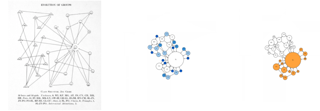
Moreno’s Sociograms (1934)

• Jacob L. Moreno Moreno (1934) pioneered social network visualization using sociograms.
• Studied classroom sociability (e.g., asking children to choose peers they would prefer to sit next to).

Micro-Level Metrics: Centrality

Degree Centrality

• Intuition: Quantifies how well-connected a node is by counting its direct connections.

• Undirected Graph: \[ \small k_i = \sum_{j=1}^{N} A_{ij} \]

• Directed Graph: \[ \small k_i^{\text{in}} = \sum_{j=1}^{N} A_{ji} \quad \text{(Inward endorsements / popularity)} \] \[ \small k_i^{\text{out}} = \sum_{j=1}^{N} A_{ij} \quad \text{(Outward activity / gregariousness)} \]

Application: Information Flow & Governance

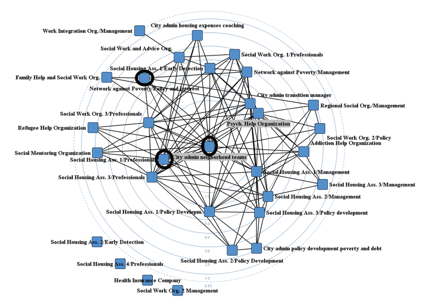
• Kenis and Raab (2020) analyzed municipality information flows.
• Without active governance interventions, communication networks spontaneously polarize into core-periphery structures, leaving peripheral actors uninformed.

Eigenvector Centrality

• Concept: A node is influential if it is connected to other highly influential nodes (recursive importance).
• Mathematical Definition: \[ \lambda x_i = \sum_{j=1}^{N} A_{ij} x_j \iff A x = \lambda x \]
• By the Perron–Frobenius theorem, for a non-negative, irreducible matrix \(A\), the dominant eigenvalue \(\lambda_1\) corresponds to an eigenvector \(x^*\) whose entries are all non-negative (\(x_i \ge 0\)).
• \(x_i^*\) represents the eigenvector centrality score of node \(i\).

Empirical Example: Lifespan Risk Trajectories

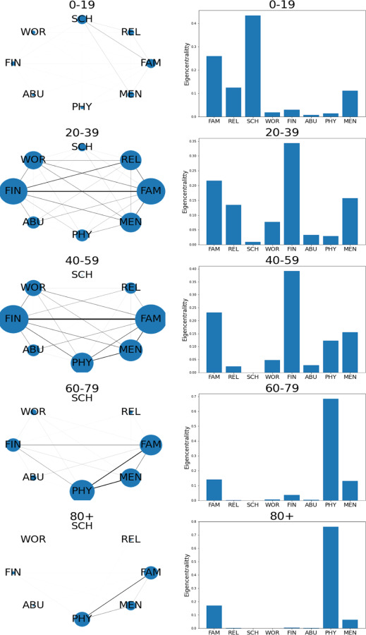
• Hsu et al. (2023) mapped risk factors and triggers across different age cohorts.
• Eigenvector centrality identifies which psychological and environmental stressors act as core drivers across developmental stages.

Betweenness Centrality

• Concept: Measures how often a node falls on the shortest path (geodesic) between other pairs of nodes—acting as a bridge or gatekeeper.

\[ C_B(i) = \sum_{s \neq i \neq t \in V} \frac{\sigma_{st}(i)}{\sigma_{st}} \]

• \(\sigma_{st}\): Total number of shortest paths between node \(s\) and node \(t\).
• \(\sigma_{st}(i)\): Number of those shortest paths passing through node \(i\).
• Applications: Information brokerage (Burt’s structural holes), organizational gatekeeping, viral super-spreaders in epidemiological models.

Computing Centrality in R and Python

• R (sna)
• Python (networkx)

library(sna)

# Create a random directed graph (10 nodes)
dat <- rgraph(10)

# In-degree, out-degree, and total degree
degree(dat, cmode = "indegree")
degree(dat, cmode = "outdegree")

# Eigenvector centrality
evcent(dat)

# Betweenness centrality
betweenness(dat)

import networkx as nx

G = nx.DiGraph()
nx.add_path(G, [0, 1, 2, 3])

# Degrees
in_deg = dict(G.in_degree())
out_deg = dict(G.out_degree())

# Eigenvector centrality
ev = nx.eigenvector_centrality(G)

# Betweenness centrality
bw = nx.betweenness_centrality(G)

Meso-Level Metrics: Communities & Clustering

Detection vs. Clustering

• Local Clustering: Evaluates local connectivity density—specifically, the probability that two neighbors of a node are themselves linked.
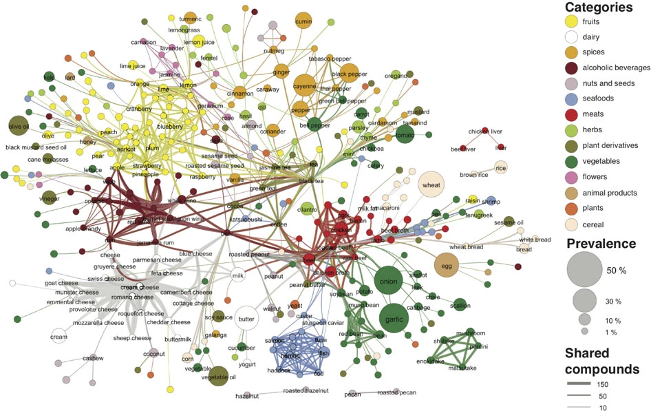
• Community Detection: Partitions the network into modular sub-units with dense internal connections and sparse inter-group connections.

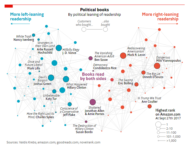
Political polarization in co-purchasing networks

Flavor pairing communities Ahn et al. (2011)

Local Clustering Coefficient

The clustering coefficient \(C_i\) of node \(i\) measures the proportion of realized ties among its \(k_i\) neighbors:

\[ C_i = \frac{2 L_i}{k_i(k_i - 1)} \]

• \(L_i\): Number of links between neighbors of node \(i\).
• \(\frac{k_i(k_i-1)}{2}\): Maximum possible links among \(k_i\) neighbors.
• Average Clustering Coefficient: \[ \langle C \rangle = \frac{1}{N} \sum_{i=1}^{N} C_i \]

Homophily & Group Boundaries

“Birds of a feather flock together”

• Definition: Tendency of nodes to form ties with similar others (based on sociodemographics, ideology, etc.).
• External-Internal (E-I) Index (Krackhardt & Stern): \[ \text{E-I} = \frac{E_{\text{external}} - E_{\text{internal}}}{E_{\text{external}} + E_{\text{internal}}} \]
  • Range: \([-1, +1]\)
  • \(-1\): Perfect homophily (all links within-group).
  • \(+1\): Perfect heterophily (all links cross-boundary).

Community Detection in Code

• R
• Python

library(igraph)

g <- sample_gnp(20, 0.15)

# Louvain modularity optimization
comm_louvain <- cluster_louvain(as.undirected(g))
membership(comm_louvain)

# Hierarchical community detection (walktrap)
comm_walktrap <- cluster_walktrap(g)

import networkx as nx

G = nx.erdos_renyi_graph(20, 0.15)

# Louvain Community Detection
communities = nx.community.louvain_communities(G)

# Greedy Modularity
greedy_comm = nx.community.greedy_modularity_communities(G)

Macro-Level Metrics & Software Ecosystem

Macro-Level Structural Dimensions

• Distance (\(d_{ij}\)): Length of the shortest path between \(i\) and \(j\).
• Network Diameter (\(D\)): Maximum geodesic distance across any connected pair: \[ D = \max_{i, j \in V} d_{ij} \]
• Average Path Length (\(\langle d \rangle\)): \[ \langle d \rangle = \frac{1}{N(N-1)} \sum_{i \neq j} d_{ij} \]
• Effective Diameter (90th percentile): Minimum distance that connects 90% of reachable node pairs (robust to outliers).

The Network Analysis Software Stack

Python

• NetworkX: Rapid prototyping & teaching
• igraph-python: High performance for large graphs
• graph-tool: C++ backend, high speed
• OSMnx: Spatial and street networks

R

• igraph: Comprehensive graph algorithms
• statnet / ergm: Statistical inference & modeling
• qgraph / bootnet: Psychometrics & partial correlation networks

GUI & Visualization

• Gephi: Interactive exploration & GPU rendering
• Cytoscape: Biological & multi-omics networks

Summary

1. Foundations: Graphs represent complex relations via nodes (\(V\)) and edges (\(E\)) encoded as adjacency matrices (\(A\)).
2. Micro Level: Degree, eigenvector, and betweenness centralities reveal distinct forms of node importance (connectivity, prestige, and brokerage).
3. Meso Level: Clustering coefficients and homophily indices capture localized social structure and modular boundaries.
4. Macro Level: Path lengths and diameters characterize how efficiently information or influence traverses the system.

Overview

• Focuses on probabilistic graphical models with applications in social science and psychology.
• Key Theoretical References:
  • Wasserman (2013), All of Statistics / Causal inference literature
  • Hastie et al. (2009) , Elements of Statistical Learning
• Software & Implementation:
  • Epskamp et al. (2012) Epskamp and Fried (2015), and Epskamp, Borsboom, and Fried (2018) psychometric network framework (qgraph , bootnet).

Graphical Models

What is a Graphical Model?

• A framework to represent joint dependency structures and relationships between random variables.
• Can be represented as:
  • Directed graphs (e.g., Bayesian networks, DAGs)
  • Undirected graphs (e.g., Markov Random Fields, partial correlation networks)

In Pursuit of Causality

• Finding causal relationships without expensive Randomized Controlled Trials (RCTs) is a primary research goal.
• RCTs are often constrained by budgets, ethical barriers, and logistics.
• The primary aim of these network graphs is to discover associations likely to indicate causal pathways.

Caveat Wasserman (2013)

RCT remains the gold standard. Any algorithmic causal discovery is an approximation reliant on structural and distributional assumptions.

Types of Network

Network	Node	Edge Meaning
Marginal Correlation Graph	Variables / Factors	Marginal correlation
Partial Correlation Graph	Variables / Factors	Conditional correlation
Conditional Independence Graph	Variables / Factors	Conditional independence
Causal Graph	Variables / Factors	Directed causation

Marginal Correlation Networks

• The most intuitive, but least informative network representation.
• Directly transforms a correlation matrix into an undirected network:
  • An edge exists between \(i\) and \(j\) if \(\text{corr}(i,j) \neq 0\) (typically evaluated via hypothesis testing).
  • Can use Pearson’s \(r\), Kendall’s \(\tau\), or Spearman’s \(\rho\).

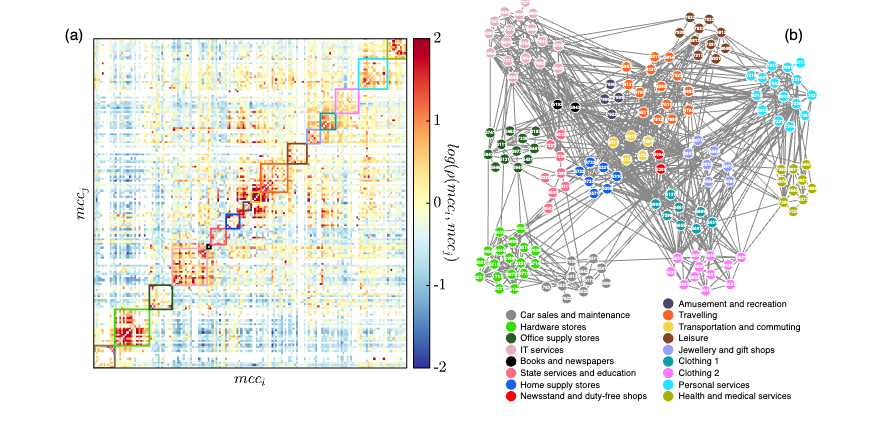
Merchant category correlation matrix and graph Leo et al. (2016)

Partial Correlation & Conditional Independence

The Need for Partial Correlation

• Marginal bivariate correlations can be spurious or explained away by third-party confounding variables.
• Partial correlation \(p(X, Y \mid Z)\):
  • Correlation between residuals \(\epsilon_X\) and \(\epsilon_Y\) after linearly regressing \(X\) on \(Z\) and \(Y\) on \(Z\).
• Connects directly to the precision matrix (inverse covariance matrix): \[\Omega = \Sigma^{-1}\]
• The partial correlation matrix entries \(R(i, j)\) are: \[R(i, j) = -\frac{\Omega_{i,j}}{\sqrt{\Omega_{i,i}\Omega_{j,j}}}\]

Conditional Independence: Gaussian Case

Let variables be jointly Gaussian: \(X \sim \mathcal{N}(\mu, \Sigma)\).

Theorem

Suppose \(X \sim \mathcal{N}(\mu, \Sigma)\). Then: \[X_i \perp \!\!\! \perp X_j \mid X_{-(i,j)} \iff \Omega_{ij} = 0\]

• In Gaussian Graphical Models (GGMs), testing for conditional independence is identical to testing if the off-diagonal elements of the precision matrix equal zero.

Categorical / Multinomial Variables

• For binary or categorical outcomes, Poisson / log-linear representations are used.
• For two binary variables \(X = (x_1, x_2)\): \[\log p(x_1, x_2) = \beta_0 + \beta_1 x_1 + \beta_2 x_2 + \beta_{12} x_1 x_2\]
• Parameter interpretations: \[\beta_{12} = \log \frac{p(0,0)p(1,1)}{p(1,0)p(0,1)}\]
• Under independence, \(\frac{p(0,1)}{p(0,0)} = \frac{p(1,1)}{p(1,0)} \implies \beta_{12} = 0\).
• Takeaway: Conditional independence corresponds to testing if the interaction/moderation parameter is zero.

Statistical Inference & Testing

Common Targets of Inference

Researchers frequently need interval estimation and hypothesis testing rather than purely point estimates:

1. Edge existence: \(A_{ij} \neq 0\)
2. Edge difference: \(A_{ij} \neq A_{jk}\)
3. Centrality differences: Node strength, closeness, betweenness

Analytical vs. Bootstrap Approaches

• Analytical / Asymptotic Methods:
  • Established by Tony Cai and his colleagues (Cai and Ma (2013),Cai and Liu (2016),Cai (2017)) for Gaussian settings.
  • Limitations: Strictly requires Gaussianity; does not readily test centrality metrics.
• The Bootstrap Solution:
  • Non-parametric or parametric resampling provides empirical distributions for:
    • Edge weights against zero (or arbitrary thresholds).
    • Confidence intervals around centrality measures and rank orderings Epskamp, Borsboom, and Fried (2018).

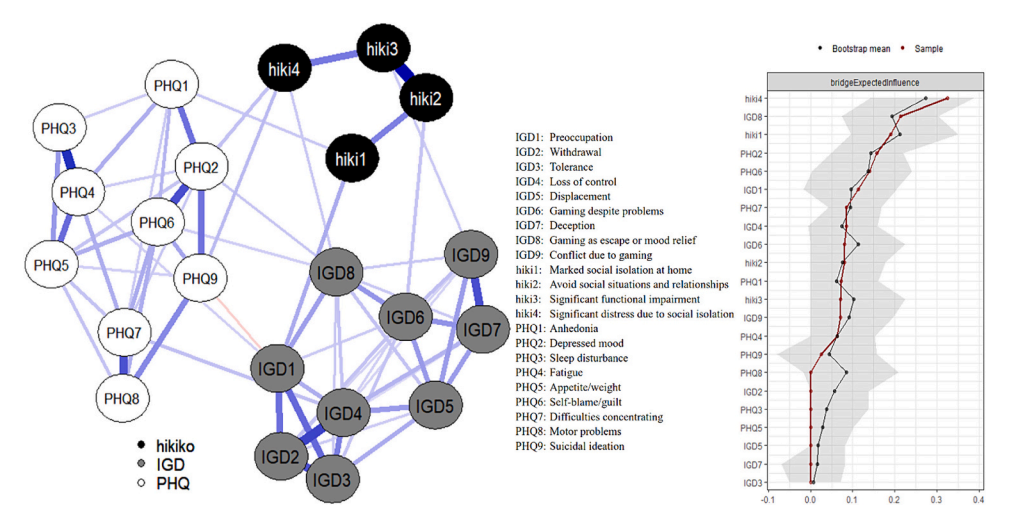
Application: Comorbidity Networks

Network showing the relation between IGD, PHQ, and social withdrawal Fong et al. (2024)

Computational Considerations

Challenges with High Dimensions

Computing empirical partial correlations directly encounters barriers:

1. Matrix Inversion: \(\Sigma^{-1}\) is unstable or non-invertible when \(p \ge n\).
2. Combinatorial Explosion: The number of conditional independence tests grows quadratically (\(\mathcal{O}(p^2)\)).

Regularization: Graphical Lasso (glasso)

• Penalizes the negative log-likelihood with an \(\ell_1\)-penalty to enforce sparsity: \[\hat{\Omega} = \arg\max_{\Omega \succ 0} \left( \ell(\Omega) - \lambda \sum_{j \neq k} |\Omega_{jk}| \right)\] where \[\ell(\Omega) = \frac{n}{2}\log|\Omega| - \frac{n}{2}\text{tr}(\Omega S_n) - \frac{nd}{2}\log(2\pi)\]
• Tuning parameter (\(\lambda\)) selection:
  • Cross-Validation (CV)
  • Extended Bayesian Information Criterion (EBIC)

Empirical Applications

Applications in Psychopathology

• Psychological symptoms can be conceptualized as interacting elements in a complex network rather than passive indicators of an unobserved latent disease entity. :::{.columns}

• Examples:
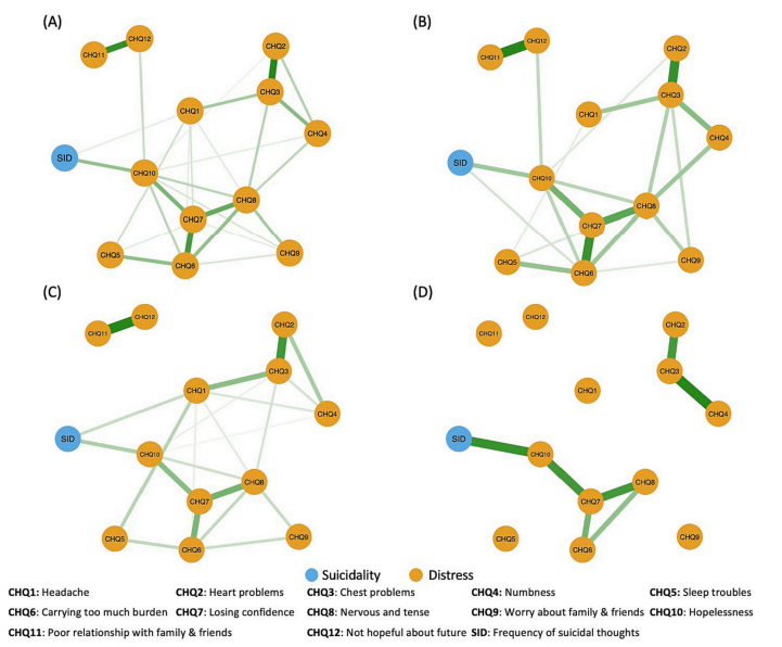
  • Depression & Suicidality: Junus and Yip (2024) demonstrated hopelessness scale items conditionally depend on suicide ideation.
  • Internet Gaming Disorder (IGD): Fong et al. (2024) identified gaming as a mood-escape mechanism directly connected to depressive mood and social withdrawal.

Hopelessness and Suicide Ideation Network Junus and Yip (2024)

:::

R Implementation

Network Estimation with bootnet

library(psychTools)
library(bootnet)
library(qgraph)

# Load sample data: Big Five Inventory (BFI)
data(bfi)
bfiSub <- bfi[, 1:25]

# 1. Marginal correlation network
Network_corr <- estimateNetwork(bfiSub, default = "cor")

# 2. Gaussian Graphical Model with EBICglasso
Network_BIC <- estimateNetwork(bfiSub, default = "EBICglasso")

# 3. Ising model for binary variables
Network_Ising <- estimateNetwork(bfiSub, default = "IsingFit")

# 4. Mixed Graphical Model (MGM) for mixed data types
Network_Mgm <- estimateNetwork(bfiSub, default = "MGM")

Visualization & Centrality Testing

# Plot network layout using the Fruchterman-Reingold algorithm
plot(Network_BIC, layout = "spring")

# Compute and plot centrality indices (Strength, Betweenness, Closeness)
centralityPlot(Network_BIC)

# Test for statistical difference in edge strength
differenceTest(Network_BIC, "A1", "C2", "strength")

Summary & Model Selection

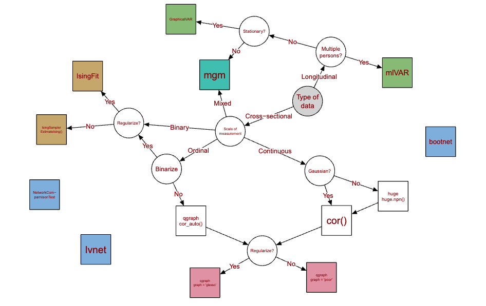
Model Selection Guidelines

Summary of network model choices (adapted from network guidelines, 2024)

• Continuous Gaussian variables: Partial correlation via EBICglasso / GGM.
• Binary variables: Ising models via IsingFit.
• Mixed variables: Mixed Graphical Models (mgm).
• Note: Continuous variables do not require an arbitrary shift between correlation and partial correlation; partial correlation graphs should generally be preferred to avoid spurious correlations.

Exponential Random Graph Models (ERGM)

Motivation for ERGMs

• Central Research Question: > Do individual attributes and local structural configurations drive the probability of tie formation?
• Empirical research requires a statistical inference framework to:
  • Estimate effect sizes (\(\beta\) / \(\theta\))
  • Calculate standard errors and \(p\)-values
  • Control for endogenous network dependencies (e.g., reciprocity, transitivity)

ERGM Problem Formulation

Let \(Y\) be an \(N \times N\) adjacency matrix of binary random variables \(Y_{ij} \in \{0, 1\}\).

The general probability distribution of observing graph \(y\) is:

\[ P(Y = y \mid \theta) = \frac{\exp\left(\theta^\top g(y)\right)}{\kappa(\theta)} \]

• \(g(y)\): Vector of network statistics (counts of edges, mutual dyads, triangles, node-level covariates).
• \(\theta\): Model parameters / coefficients to estimate.
• \(\kappa(\theta) = \sum_{y^* \in \mathcal{Y}} \exp\left(\theta^\top g(y^*)\right)\): Intractable normalizing constant summing over all \(2^{\binom{N}{2}}\) possible networks.

Local Conditional Interpretation: Change Statistics

Conditioning on the rest of the network (\(Y_{-ij}\)), the log-odds of a tie between \(i\) and \(j\) takes a logistic form:

\[ \text{logit}\left(P(Y_{ij} = 1 \mid Y_{-ij}, \theta)\right) = \theta^\top \delta(y)_{ij} \]

where \(\delta(y)_{ij}\) is the change statistic:

\[ \delta(y)_{ij} = g\left(y_{ij}^{+}\right) - g\left(y_{ij}^{-}\right) \]

• \(y_{ij}^{+}\): The network with edge \((i, j)\) present.
• \(y_{ij}^{-}\): The network with edge \((i, j)\) absent.

Structural Elements of \(g(y)\)

1. Dyadic Independent Terms:
   • Density: Number of edges \(\sum y_{ij}\)
   • Nodal Covariates: Main effects of sender/receiver attributes (e.g., age, gender)
   • Dyadic Covariates: Homophily / absolute difference \(|X_i - X_j|\)
2. Dyadic Dependent Terms (Endogenous Structures):
   • Reciprocity: Mutual ties \(\sum y_{ij} y_{ji}\)
   • Triadic Closure: Triangles, transitive ties
   • Degree Distributions: Star terms, Geometrically Weighted Degree (GWESP, GWDegree)

Practical Estimation in R (statnet) Handcock et al. (2008)

Dataset: Bott (1928) Children Imitation

• Adopted from Robins et al. (2007)
• Observational study of children’s playgroup behaviors (Bott, 1928).
• A directed edge from \(i \to j\) indicates child \(i\) imitated child \(j\).
• Analyzed in Bott’s 4th observation group (\(N = 11\), total possible directed dyads \(= 11 \times 10 = 110\)).

library(networkdata)
library(statnet)
data(bott)

# Inspect network and observed edge count
summary(bott[[4]] ~ edges)
## edges 
##    35

Baseline Model: Bernoulli Random Graph

bottmodel.01 <- ergm(bott[[4]] ~ edges)
summary(bottmodel.01)

## ==========================
## Monte Carlo MLE Results:
##       Estimate Std. Error MCMC %  p-value    
## edges  -0.7621     0.2047      0 0.000313 ***
## ---
## Residual Deviance: 137.6 on 109 degrees of freedom
## AIC: 139.6   BIC: 142.3

• Interpretation: \[\text{logit}(p) = -0.7621 \implies p = \frac{1}{1 + e^{0.7621}} \approx 0.318 = \frac{35}{110}\]
• This recovers the observed density directly via maximum likelihood.

Adding Nodal Attributes (In-Degree Covariate)

Hypothesis: Are older children imitated more frequently (higher in-degree)?

bottmodel_node <- ergm(bott[[4]] ~ edges + nodeicov('age.month'))
summary(bottmodel_node)

##                    Estimate Std. Error MCMC % p-value   
## edges              -2.89853    0.96939      0 0.00345 **
## nodeicov.age.month  0.05225    0.02272      0 0.02340 * 

• Conditional Log-Odds: \[\text{logit}(P(Y_{ij}=1)) = -2.90 + 0.052 \times (\text{Age of child } j)\]
• Effect:
  • For a 36-month-old target: \(-2.90 + 0.052(36) = -1.028 \implies P \approx 0.263\)
  • For a 48-month-old target: \(-2.90 + 0.052(48) = -0.404 \implies P \approx 0.400\)

Adding Endogenous Structural Terms: Triangles

Triangles quantify transitivity and local clustering:

bottmodel_triangle <- ergm(bott[[4]] ~ edges + triangle)
summary(bottmodel_triangle)

##          Estimate Std. Error MCMC % p-value
## edges    -0.55772    0.58201      0   0.340
## triangle -0.05674    0.15330      0   0.712

• Conditional Log-Odds: \[\text{logit}(P(Y_{ij} = 1 \mid Y_{-ij})) = -0.558 - 0.057 \times (\Delta \text{Triangles})\]
  • Tie creates 0 triangles: \(-0.558 - 0.057(0) = -0.558\)
  • Tie creates 1 triangle: \(-0.558 - 0.057(1) = -0.615\)
  • Tie creates 2 triangles: \(-0.558 - 0.057(2) = -0.672\)

Estimation & Model Diagnostics

Why Standard Logistic Regression Fails

• Standard GLMs assume independent observations (\(Y_{ij} \perp \!\!\! \perp Y_{kl}\)).
• In networks with structural terms (e.g., triangle):
  • Whether tie \((i, j)\) forms a triangle depends on \((i, k)\) and \((k, j)\).
  • Dyadic dependence violates the \(i.i.d.\) assumption.
• The normalizing constant \(\kappa(\theta) = \sum_{y^*} \exp(\theta^\top g(y^*))\) cannot be computed analytically (\(2^{\binom{N}{2}}\) states).
• Solution: Markov Chain Monte Carlo Maximum Likelihood Estimation (MCMLE) via Metropolis–Hastings sampling.

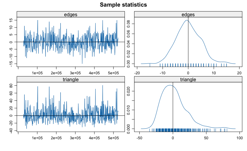
MCMLE Diagnostics

library(latticeExtra)
mcmc.diagnostics(bottmodel_triangle)

• Trace Plots: Should fluctuate stably around zero (white noise).
• Density Plots: Should be centered at 0 and approximately bell-shaped.
• Autocorrelation: Should decay rapidly toward zero as lag increases.
• Geweke Diagnostic: Checks difference between early and late parts of the chain (\(p > 0.05\) indicates stationary convergence).

Model Degeneracy

Caution on Naive Triangle Terms

Models with raw triangle counts frequently suffer from MCMC degeneracy: - The simulated chain collapses into either a completely empty graph or a complete clique. - Standard errors blow up, or MCMLE fails to converge.

• Modern Solution: Use geometrically weighted terms with decreasing marginal returns:
  • gwesp (Geometrically Weighted Edgewise Shared Partner)
  • gwdgree / gwidegree / gwodegree

Goodness of Fit (GOF)

We evaluate whether the fitted model reproduces higher-order network metrics not explicitly parameterized: Hunter, Goodreau, and Handcock (2008)

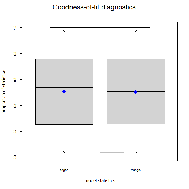
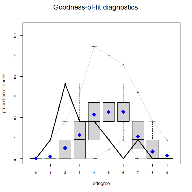
bottmodel_triangle_gof <- gof(bottmodel_triangle ~ model + odegree)
plot(bottmodel_triangle_gof)

• Solid line = Observed network value.
• Boxplots = Values across networks simulated from fitted \(\hat{\theta}\).
• If the observed line sits within the simulation intervals, the model fits well.

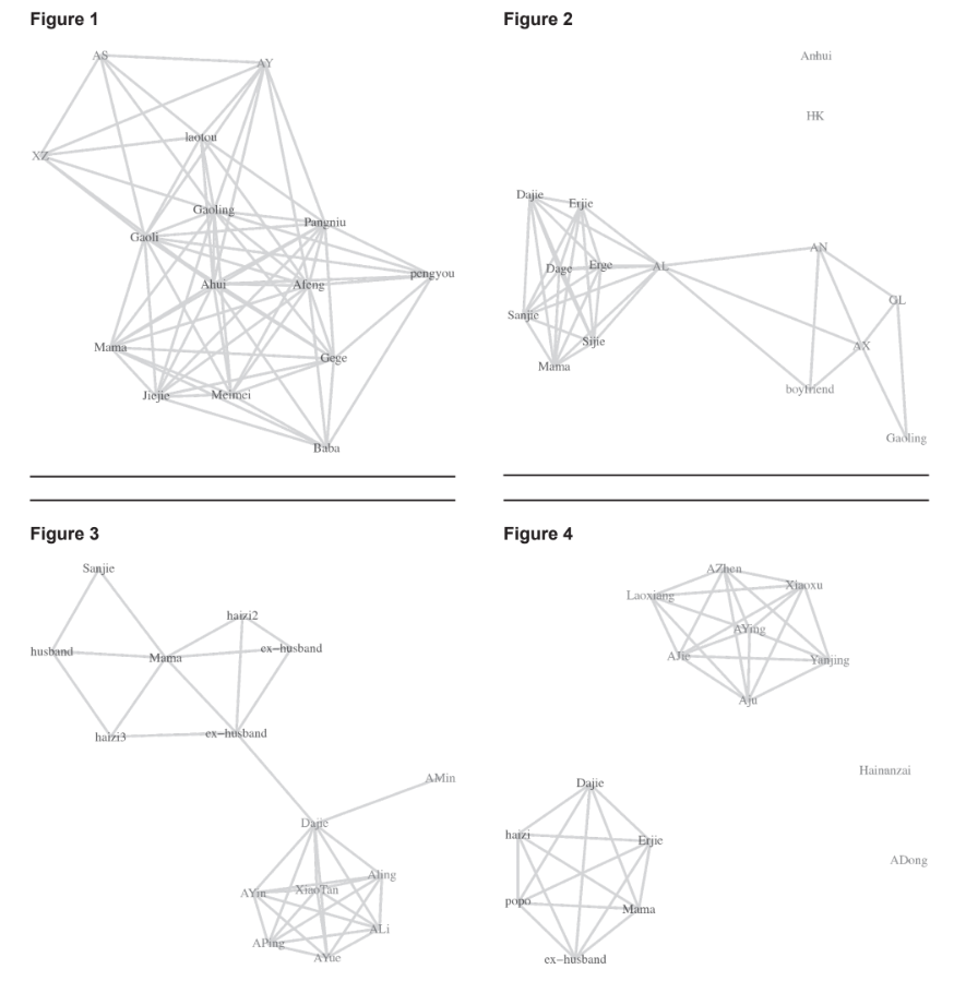
Real-World Application

• Network Study: Female sex worker network in Hainan Province Yu et al. (2016).
• Structural Findings:
  • High transitivity and clustering within subgroups facilitated mutual safety and peer education.
  • However, customer contact networks showed structural holes due to economic competition.

Summary

1. Random Graphs as Null Models:
   • ER graphs establish a baseline for completely random tie formation.
   • Small-world (WS) and Scale-free (BA) models highlight mechanisms producing high clustering and hubs.
2. ERGMs for Hypothesis Testing:
   • Model the full joint distribution of a network.
   • Change statistics evaluate individual attributes and local structural configurations simultaneously.
3. Robust Practice:
   • Always verify MCMC convergence (mcmc.diagnostics).
   • Guard against degeneracy using tapered terms (gwesp).
   • Confirm out-of-model fit via gof().

Refernce list

Ahn, Yong-Yeol, Sebastian E Ahnert, James P Bagrow, and Albert-László Barabási. 2011. “Flavor Network and the Principles of Food Pairing.” Scientific Reports 1 (1): 196.

Barabási, Albert-László. 2013. “Network Science.” Philosophical Transactions of the Royal Society A: Mathematical, Physical and Engineering Sciences 371 (1987): 20120375.

Cai, T Tony. 2017. “Global Testing and Large-Scale Multiple Testing for High-Dimensional Covariance Structures.” Annual Review of Statistics and Its Application 4 (1): 423–46.

Cai, T Tony, and Weidong Liu. 2016. “Large-Scale Multiple Testing of Correlations.” Journal of the American Statistical Association 111 (513): 229–40.

Cai, T Tony, and Zongming Ma. 2013. “Optimal Hypothesis Testing for High Dimensional Covariance Matrices.”

Epskamp, Sacha, Denny Borsboom, and Eiko I Fried. 2018. “Estimating Psychological Networks and Their Accuracy: A Tutorial Paper.” Behavior Research Methods 50: 195–212.

Epskamp, Sacha, Angélique OJ Cramer, Lourens J Waldorp, Verena D Schmittmann, and Denny Borsboom. 2012. “Qgraph: Network Visualizations of Relationships in Psychometric Data.” Journal of Statistical Software 48: 1–18.

Epskamp, Sacha, and Eiko I Fried. 2015. “Package ‘Bootnet’.” Bootstrap Methods for Various Network Estimation Routines 5: 0–1.

Fong, Ted CT, Alvin Junus, Ming Wen, and Paul SF Yip. 2024. “Comorbidity Among Symptoms of Internet Gaming Disorder, Social Withdrawal, and Depression in 3430 Young People in Hong Kong: A Network Analysis.” Journal of Affective Disorders 359: 319–26.

Handcock, Mark S, David R Hunter, Carter T Butts, Steven M Goodreau, and Martina Morris. 2008. “Statnet: Software Tools for the Representation, Visualization, Analysis and Simulation of Network Data.” Journal of Statistical Software 24 (1): 1548.

Hastie, Trevor, Robert Tibshirani, Jerome H Friedman, and Jerome H Friedman. 2009. The Elements of Statistical Learning: Data Mining, Inference, and Prediction. Vol. 2. Springer.

Hsu, Yu Cheng, Alvin Junus, Qingpeng Zhang, Clifford Wong, Tsz Mei Lam, Florence Cheung, Joyce Liu, Ingrid D Lui, and Paul SF Yip. 2023. “A Network Approach to Understand Co-Occurrence and Relative Importance of Different Reasons for Suicide: A Territory-Wide Study Using 2002–2019 Hong Kong Coroner’s Court Reports.” The Lancet Regional Health–Western Pacific.

Hunter, David R, Steven M Goodreau, and Mark S Handcock. 2008. “Goodness of Fit of Social Network Models.” Journal of the American Statistical Association 103 (481): 248–58.

Junus, Alvin, and Paul SF Yip. 2024. “Evaluating Potential Effects of Distress Symptoms’ Interventions on Suicidality: Analyses of in Silico Scenarios.” Journal of Affective Disorders 347: 352–63.

Kenis, Patrick, and Jörg Raab. 2020. “Back to the Future: Using Organization Design Theory for Effective Organizational Networks.” Perspectives on Public Management and Governance 3 (2): 109–23.

Leo, Yannick, Márton Karsai, Carlos Sarraute, and Eric Fleury. 2016. “Correlations of Consumption Patterns in Social-Economic Networks.” In 2016 IEEE/ACM International Conference on Advances in Social Networks Analysis and Mining (ASONAM), 493–500. IEEE.

Menczer, Filippo, Santo Fortunato, and Clayton A. Davis. 2020. A First Course in Network Science. Cambridge University Press. https://doi.org/10.1017/9781108653947.

Mondrian, Piet. 1942. Broadway Boogie Woogie. Oil on canvas. The Museum of Modern Art.

Moreno, Jacob Levy. 1934. “Who Shall Survive?: A New Approach to the Problem of Human Interrelations.”

Newman, Mark. 2018. Networks. Oxford university press.

Robins, Garry, Pip Pattison, Yuval Kalish, and Dean Lusher. 2007. “An Introduction to Exponential Random Graph (p*) Models for Social Networks.” Social Networks 29 (2): 173–91.

Wasserman, Larry. 2013. All of Statistics: A Concise Course in Statistical Inference. Springer Science & Business Media.

Yu, Yeon Jung, Christopher McCarty, James Holland Jones, and Xiaoming Li. 2016. “In-Transitivity: Network Patterns of Female Sex Workers (FSWs) in China.” Human Organization 75 (4): 358–70.